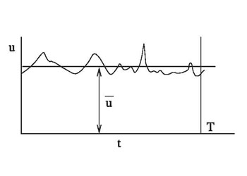
Equation (i) is called the ensemble average of  . Equation (ii) is based on a linear fit for . Equation (ii) is based on a linear fit for  between successive points. Equation (i) is usually preferred over (ii) because it under-predicts the value of the integral and de-emphasizes the occurrence of isolated peak values. between successive points. Equation (i) is usually preferred over (ii) because it under-predicts the value of the integral and de-emphasizes the occurrence of isolated peak values.

Figure 1.8: Sketch of a Random Signal. |
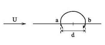
The integrals appearing above are quite sensitive to the choice of  (and hence (and hence  ), namely the total time of data collection. While the desired value of ), namely the total time of data collection. While the desired value of  can be estimated by increasing the length of the signal till the mean and RMS values converge to values that are independent of can be estimated by increasing the length of the signal till the mean and RMS values converge to values that are independent of  , this is not very convenient. One can estimate the value of , this is not very convenient. One can estimate the value of  from the physics of the problem being studied. Consider atmospheric flow as an example. There will be fluctuations arising from the motion of eddies of a variety of sizes that are transported by the flow. The fluctuation due to a typical eddy is schematically shown in Figure 1.9. from the physics of the problem being studied. Consider atmospheric flow as an example. There will be fluctuations arising from the motion of eddies of a variety of sizes that are transported by the flow. The fluctuation due to a typical eddy is schematically shown in Figure 1.9.

Figure 1.9: Model of an Eddy to Define Time Scales in the Flow. |
|