Figure 4.68 is an expanded view of the wedge fringes. Let us find concentration (of a solute in a solution or change in temperature from a reference value in a physical domain) at any point in the interferogram. The deviation of fringe 2 near the crystal-solution interface is , while at any other point, it is denoted as . Since fringe displacement relates linearly with change in phase, hence refractive index and material density, we can write

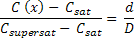
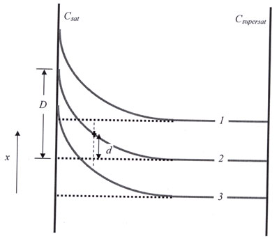
Figure 4.68: Computing concentration in the presence of the wedge fringes

Since all other parameters except are known, the local concentration can be easily calculated. The concentration gradient is obtained from the slope of the fringes at a point . The above methodology is used for calculating the concentration at points which lie on the wedge fringes. However, if one were to find concentration at a point lying between two wedge fringes, instead of on them, then one has to locate four nearby points on the wedge fringes and compute their respective concentrations. It is then followed by using a suitable interpolation technique to find the concentration at the desired point.

Concentration data over a uniform grid

Once the absolute concentration corresponding to the fringes (in the wedge as well as infinite fringe setting) has been computed, the irregularly spaced concentration data must be transferred to a two-dimensional uniform grid over the fluid region. This is necessary to enable application of the tomographic algorithms for reconstruction of the three-dimensional concentration field. For this purpose, a two-dimensional linear interpolation procedure is followed by superimposing a 2D grid over the thinned interferograms. After completing the interpolation procedure, the equi-concentration contours are plotted. These contours should closely follow the originally recorded fringe pattern. It works as a cross-check for the data obtained after interpolation and provides an estimate of the interpolation errors.