ART
Various ART algorithms are available in the literature owing their origin to Kacz-marz [95] and Tanabe [96]. They differ from each other in the way the correction is applied. Those presented below have been tested successfully by the author and his coworkers in the context of interferometry.
Simple ART
This algorithm has been suggested by Mayinger [6]. The corrections are applied through a weight factor. Computed as an average correction along a ray. The deference between the calculated projections with the measured projection data gives the total correction to be applied for a particular ray. The average correction is then the contribution to each cell falling in the path of the ray. This is computed by dividing the total correction obtained with the length of the ray. The calculated projection are computed once for a particular angle. Though are field values are continuously updated the calculated projection values remain unchanged until the completion of all the rays for a given angle. This algorithm will be referred to as ART1 in future discussions.
Let  be the projection due to the be the projection due to the  -th ray in the -th ray in the  direction of projection and direction of projection and  be the initial guess of the field value. Numerically the projection be the initial guess of the field value. Numerically the projection  using the current field values is defined as: using the current field values is defined as:
The individual steps in the algorithm are listed below.
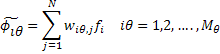
Calculate the total value of weight function  along each ray as: along each ray as:
Start: 1 For each projection angle 
Start:2 For each ray 
Start:3 For each cell 

Close:3
Close:2
Close:1
|