Figure 4.29 shows the local Nusselt number variation with the coordinate over one roll for the three thinning algorithms. Both the hot and cold walls have been considered. The view angle is 90 degrees and so the roll formation is visible in this projection. The roll angle is 90 degrees and so the roll formation is visible in this projection. The roll being inclined, the Nusselt number variation on the two walls are of opposite orientation. The three thinning algorithms qualitatively reproduce these trends. The Nusselt number profile predicted by the automatic thinning algorithm can be seen to be the smoothest of the three. Differences among the three algorithms can be seen to have increased in Figure 4.29, compared to the errors reported in Table 2. This is because the Nusselt number calculated form the three algorithms are within of one another.
Figure 4.29: Local Nusselt number variation over the hot and cold paltes; comparision of the three thinning algorithms
Table 4 presents the Nusselt number averaged over a single roll in the fluid layer. The automatic fringe thinning algorithm gives Nusselt number that are comparatively close on the two walls. For the zero degrees projection, the average Nusselt number over the two plates differs for both the curve–fitting and the paintbrush methods. The roll in the present study is seen to be formed parallel to the zero degrees axis. These is a considerable mismatch in the average Nusselt number over a single roll as viewed along the projection data. The cavity-averaged Nusselt number however, is close to the predictions of Gebhart et al. [89]
Table 4: Comparison of Average Nuselt Number Based on the width-averaged temperature
 coordinate over one roll for the three thinning algorithms. Both the hot and cold walls have been considered. The view angle is 90 degrees and so the roll formation is visible in this projection. The roll angle is 90 degrees and so the roll formation is visible in this projection. The roll being inclined, the Nusselt number variation on the two walls are of opposite orientation. The three thinning algorithms qualitatively reproduce these trends. The Nusselt number profile predicted by the automatic thinning algorithm can be seen to be the smoothest of the three. Differences among the three algorithms can be seen to have increased in Figure 4.29, compared to the errors reported in Table 2. This is because the Nusselt number calculated form the three algorithms are within
  of one another.
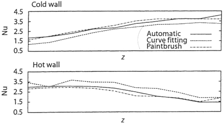
 projection data. The cavity-averaged Nusselt number however, is close to the predictions of Gebhart et al. [89]


