Temperature calculation

Each pair of fringes represents a temperature shift of . In a region subjected to an overall temperature difference of , the number of fringes to appear in the field of view can be estimated as . A fringe may be lost in the rounding process and is to be connected to the fact that walls may be isotherms but not necessarily a site for fringe formation where the phase difference must satisfy the condition of destructive interference. The spacing between fringes will depend on the temperature gradient prevailing at that location. The entire information about temperature values, localized at the fringes and the boundary of the material domain can be mapped on to a grid by a suitable interpolation procedure.

Let be the wall temperature and , the temperature of the fringe next to it. Let represent the distance between the fringe and the wall; in most applications, will be spatially distributed and not be a constant. Near a wall, the heat flux exchanged by the surface with the fluid can be calculated as

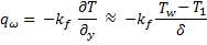
Fringe patterns recorded by a Mach-Zehnder interferometer are shown in figure 4.8. Wedge fringes and Michelson interferometry are discussed in Lecture 25.

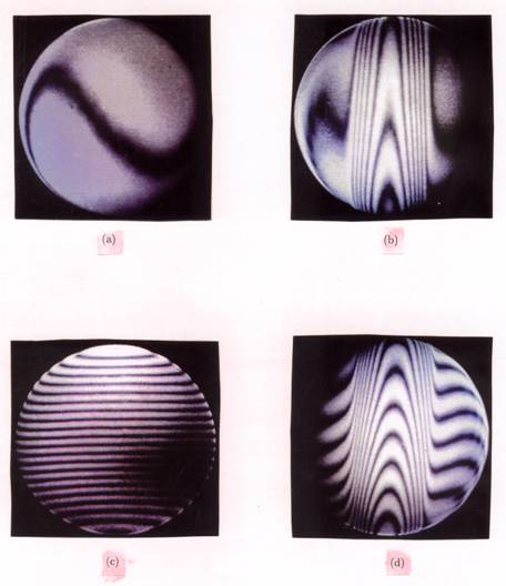
Figure 4.8: Fringes recorded above a Candle Flame in an Infinite Fringe Setting (left) and the Wedge Fringe Setting (right)