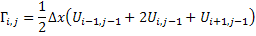
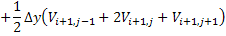
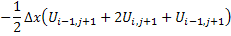
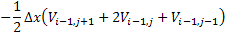
In the present work, vorticity has been calculated by choosing a small rectangular contour around which the circulation is calculated from the velocity field using a numerical integration scheme, such as trapezoidal rule. The local circulation is then divided by the enclosed area to arrive at an average vorticity for the sub-domain. The following formula provides a vorticity estimate at a point (i; j) based on circulation using eight neighboring points (see Figure 3.32):

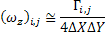
with

It has been observed from experiments that a circulation calculation via the velocity field yields better estimates of vorticity, and in particular, the peak vorticity that is otherwise under-predicted. At other locations, the vorticity field determined by the two approaches are practically identical. The accuracy of the vorticity measurement from PIV data depends on the spatial resolution of the velocity sampling and the accuracy of the velocity measurements. Therefore, the vorticity error can be associated with calculation scheme and the grid size used for velocity sampling. Another source of uncertainty is that propagated from the velocity measurements. PIV velocity measurements are the local averages of the actual velocity in the sense that it represents a low pass filtered version of the actual velocity field. Thus, vorticity from PIV data is only a local average of an already averaged velocity field and not a point measurement.