MAC Formulation

The region in which computations are to be performed is divided into a set of small cells having edge lengths and (Fig. 32.1).

Figure 32.1: Discretization of a three-dimensional domain.

With respect to this set of computational cells, velocity components are located at the centre of the cell faces to which they are normal and pressure and temperature are defined at the centre of the cells. Cells are labeled with an index which denotes the cell number as counted from the origin in the and directions respectively. Also is the pressure at the centre of the cell , while is the x-direction velocity at the centre of the face between cells and and so on (Fig. 32.2).

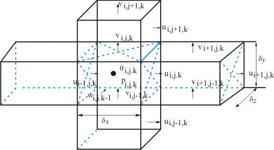
Figure 32.2: Three-dimensional staggered grid showing the locations of the discretized variables.

Because of the staggered grid arrangements, the velocities are the nodal points, but whenever required, they are to be found by interpolation. For example, with uniform grids, we can write Where a product or square of such a quantity appears, it is to be averaged first and then the product to be formed.