On the solid surface  the vorticity is certainly not zero. Here, the wall vorticity has to be derived in the same way as in the backward facing step problem. Starting with Equation (26.1) and incorporating the impervious and no-slip conditions of the vorticity is certainly not zero. Here, the wall vorticity has to be derived in the same way as in the backward facing step problem. Starting with Equation (26.1) and incorporating the impervious and no-slip conditions of  and and  (or alternatively, (or alternatively,  and and  for all for all  ), the expression for the wall vorticity reduce to ), the expression for the wall vorticity reduce to
Now, the wall vorticity can be calculated using the image point method.

Figure 26.2: Finite Difference Grid for Flow Over a Cylinder
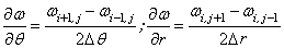
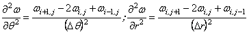
Considering a curvilinear grid as shown in Figure 26.2, the derivatives of steam function or vorticity can be replaced by their discrete (central difference) forms as:
Similarly, expressions for stream function derivatives can also be obtained. Substituting these expression into the governing equations (26.1) and (26.2) the nodal equations of all interior nodes (  ) are derived. Finally, the set of discretized equation and boundary conditions are solved by iterative methods. For high Reynolds number flows, upwinding can also be implemented based on the magnitudes of ) are derived. Finally, the set of discretized equation and boundary conditions are solved by iterative methods. For high Reynolds number flows, upwinding can also be implemented based on the magnitudes of  and and  in a similar manner as described earlier. in a similar manner as described earlier.
The important fact to be kept in mind while simulating flows in curvilinear geometries is that due to curvature, certain terms in the governing equation or boundary conditions may take a  form. In such cases, one can either resolve the form. In such cases, one can either resolve the  form using let L' Hospital rule (if possible) or employ a local cartesian mesh at the point of singularity. form using let L' Hospital rule (if possible) or employ a local cartesian mesh at the point of singularity. |