9.1 Hugoniot Curve

We have understood the typical Hugoniot curve in Figure 8.1. As per the Hugoniot curve, there are many possible states behind the shock for a given initial condition. Therefore, knowledge of massflux or Mach number is necessary to arrive at a perticular state . A straight line of the slope proportional to the massflux or Mach number when drawn along with Hugoniot curve, gives a fixed state behind the normal shock for known upstream state properties. The point at which this straight line cuts the Hugoniot curve corresponds to the state behind the shock. Possibility of such a state is still unclear since the procedure for finding the post shock condition is based on Hugoniot relation which in turn is based on mass, momentum equations and first law of thermodynamics. The straight line equation is also based on mass and momentum equations only. Therefore to select a possible state for a given initial conditions and known massflux, we have to use second law of thermodynamics. Here we can prove the impossibility of expansion shock and presence of shock in supersonic and hypersonic flows.
We know that the Hugoniot equation is



Since we know properties at station 1 therefore these can be treated as constants in this equation.



Differentiating above equation


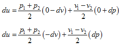
We can assume that there is a reversible heat addition process in a closed system for which we will have same initial and final states as that of the normal shock. Therefore the internal energy and entropy change for assumed process will be same as that of the normal shock case. Lets apply laws of thermodynamics to the assumed process.

dQ = du + pdv
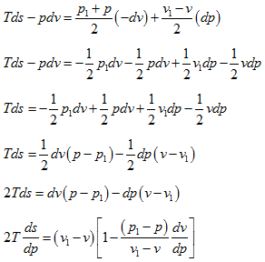
Tds = du + pdv
du = Tds - pdv
Since change in internal energy is same for both the processes, let’s equate the change in internal energy after removing subscript 2 we get,

9.1

Here T is the temperature at which heat is added reversibly to the assumed process. But we are overlapping the normal shock with the assumed reversible heat addition process. However, from combination of mass and momentum equation we have already derived the slope for normal shock in terms of massflow rate. The same thing is mentioned herewith in short.

Mass flux = pv = p1v1 = p2v2 = constant = k

9.2

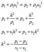
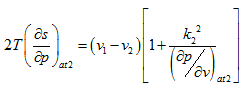
This is the slope of the straight line drawn to intersect Hugoniot curve. Using above expression, we can re-write equation (9.1) as,

9.3

Since derivatives in the above expression are of the properties of system which can belong to any process (normal shock or reversible heat addition).

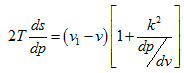
Fig 9.1: Analysis of normal shock using Hugoniot Curve

The above figure will help us in finding most probable post shock condition. In this figure, along with Hugoniot curve, three different lines are drawn to get various possible post shock conditions. These lines correspond to different massflow rates or freestream conditions forming the normal shock. One of those lines is tangent to Hugoniot curve at point 1 which represents the initial condition or pre-shock conditions. Hence the straight line at point 1 has slope (-k₁²) which is same as the Hugoniot curve at that point, . Therefore term in bracket of eq. (9.3), becomes 2. However, (v₁ - v) is equal to zero since there is no change in specific volume. Therefore is equal to zero intern dS is equal to zero which makes this process possible.

Now consider the line with slope k₂² intersecingt at point 2 to Hugoniot curve. For this case right hand side of eq. (9.3) can be written as,

9.4

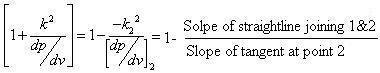
Equation (9.3) for the correcponding line can be written as,

9.5