Module 5 : Fluid Film Lubrication

Interpretation of Reynolds Equation for Incompressible Lubricants

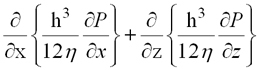
Reynolds’ Equation for incompressible lubricants :

....Eq.(5.22)

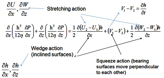
• Left hand side term is called pressure term. • Right hand side terms are called source terms. • ∂U/ ∂x , ∂W/∂z :- Called stretching action. • ∂h/∂x , ∂h/∂z :- Wedge action(inclined surfaces). • (V1 - V2) :- Squeeze action(bearing surfaces move perpendicular to each other).

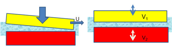
Fig. 5.10: Description of Reynolds equation.

If surface is very soft and stretchable, then velocity gradient on the surface of bearing(as shown in Fig. 5.11) occurs.

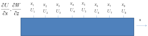
Fig. 5.11: Streching action.

Reynolds equation(Eq.5.22) can be simplified by making few assumptions. Assuming constant viscosity(η)

Assuming no relative velocity in Z-direction (W1 = W2 = 0).

...Eq.(5.23)

Equation(5.23) is applicable for following assumptions : 1. Negligible inertia terms 2. Negligible pressure gradient in the direction of film thickness 3. Newtonian fluid 4. Constant value of viscosity 5. No slip at liquid solid boundary 6. Neglecting angle of inclination for coordinate system 7. Incompressible flow 8. Relative tangential velocity only in x-dir

Assuming no stretching action.

Assuming one surface with zero tangential velocity.

....Eq.(5.24)

Equation 5.24 is applicable for following assumptions : 1. Negligible inertia terms 2. Negligible pressure gradient in the direction of film thickness 3. Newtonian fluid 4. Constant value of viscosity 5. No slip at liquid solid boundary 6. Neglecting angle of inclination for coordinate system 7. Incompressible flow 8. Relative tangential velocity only in x-dir 9. Both rigid surfaces 10. Only inclined surface slides

Pressure Distribution :

To estimate fluid film pressure, Reynolds equation(5.25) needs to be solved. Easiest way to solve this equation is to neglect pressure distribution in one direction and consider pressure gradient only in one direction(as shown in Fig. 5.12 and Fig. 5.13). Other method is numerical method in which non-dimensionalization of cordinates and fluid pressure is required for getting faster convergence of solution.

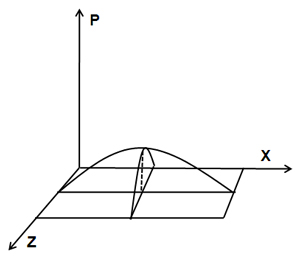
Fig. 5.12: Dimension in x-dir is much larger than dimension in z-dir

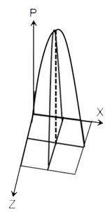
Fig. 5.13: Dimension in z-dir is much larger than dimension in x-dir

....Eq.(5.25)

On non-dimensionlizing 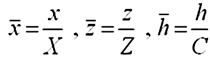in terms of Reynolds equation such as

On non-dimensionlizing Eq.(5.25)

Or ..

On substituting non dimensional pressure and time, Reynolds equation becomes Eq.(5.26).

....Eq.(5.26)

Where two most common approximations are "short bearing" and "long bearing".

....Eq.(5.27)

....Eq.(5.28)

Equation 5.27 shows that pressure gradient in X - direction is neglegible, while Eq.(5.28) shows that pressure gradient in Z - direction is negligible. In other words effect of terms in the Reynolds’ equation depends on the geometry of the bearings.

Solution of Steady State Reynolds’ Eq. :

In static case, Journal position remains in static equilibrium and film thickness remains constant w.r.t time. In other words, ∂h/∂t term of Eq.(5.26) will be zero and equation reduces to Eq.(5.27).

....Eq.(5.29)

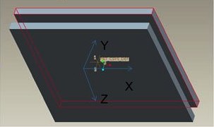
Fig. 5.14(a): Tribo surfaces under full film lubrication.

To solve Eq.(5.29) for tribo surface[Fig. 5.14(a)], surface can be discrelized in number of nodes, as shown in Fig. 5.14(b).

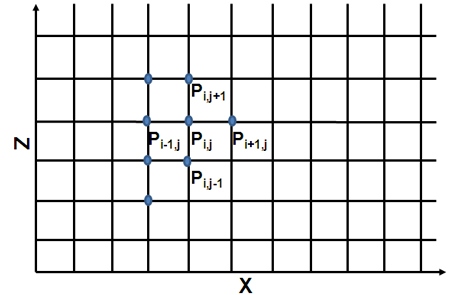
Fig. 5.14(b): Discretization of surface.

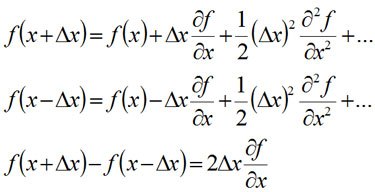
To approximate partial derivation following Tayler series can be utilized.

This means.. 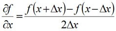....Eq.(5.30)

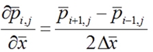....Eq.(5.31)

and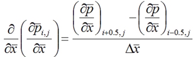

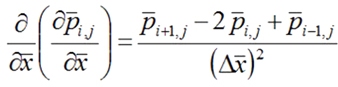....Eq.(5.32)

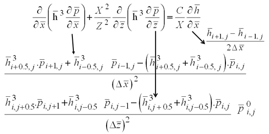
Using this kind of Taylor series approximation in Eq.(5.29).

On rearranging

....Eq.(5.33)

Eq.(5.33) can be solved for i = 1, N and j = 1, M with appropriate boundary conditions, by writing sequence of equations, such as

As most of values of nodal pressures(pi,j) are unknown therefore iterative loop is employed to estimate the fluid prerssure.

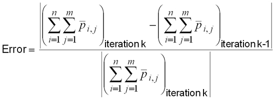
Process of iterations will be repeated till following a convergence criterion is satisfied.

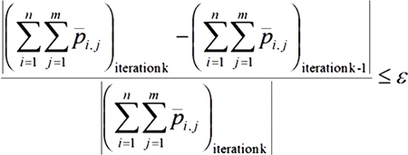....Eq.(5.34)

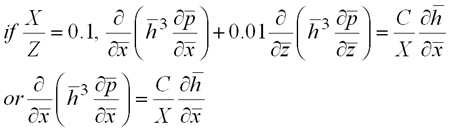
The value of ε is very small. To understand complexity of solving Eq.(5.33), let us assume N = 25, m = 25, k = 30. This means number of required steps 25 * 25 * 30 --> 18750. Calculation can be reduced by approximating short length compared to other direction as given in Eq.(5.35) if transverse Z length of surface is much lesser than tangential(X) length. By this approximate gradient is one direction(X) direction is negligible.

....Eq.(5.35)

N = 0, m = 25, k = 15. Number of required steps 25 * 15 --> 375. 18750/375 = 50 times !!! --> This means number of calculations decrease significantly by making short-bearing approximation.

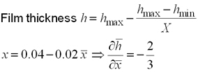
Example : Assume a thrust pad of 10*100 mm dimensions. Leading and trailing film thicknesses are 0.04 and 0.02 mm respectively. Sliding speed is 20 m/s. Viscosity of oil is 10 mPa.s. Find pressure distribution.

Average clearence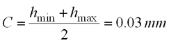

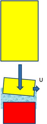
Fig. 5.15: Tangential length much lesser than transverse length.

Non dimensional film thickness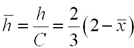

....Eq.(5.37)

On rearranging 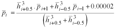....Eq.(5.38)

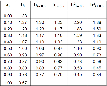
As film thickness is based on geometry, which does not change with time and iterations, therefore film thickness can evaluated and stored as listed in Table 5.1.

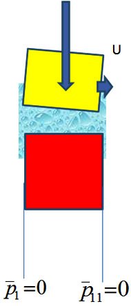
Fig. 5.16: Boundary condition.

Table 5.1: Film thickness values.

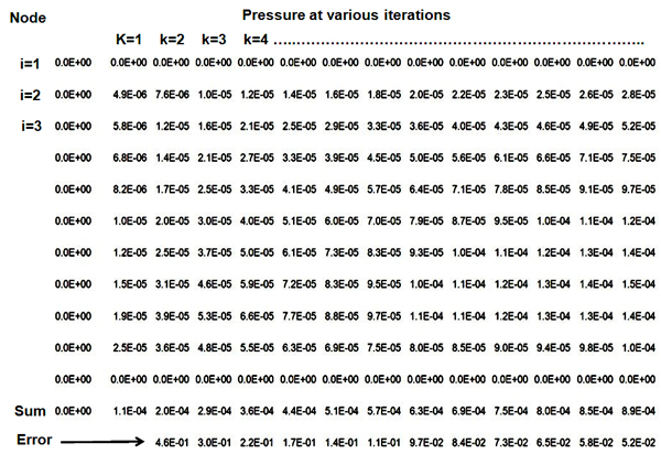
Using the values of film thickness(Table 5.1) and Eq.(5.38), pressure at various iterations can be evaluated as listed in Table 5.2. Over every iteration error(Eq.5.39) shall reduce. In the present example error at second iteration is 0.46 and error at 13 iteration is 0.052 as given in Table 5.2.

Table 5.2: Values of fluid pressure over iterations.

....Eq.(5.39)

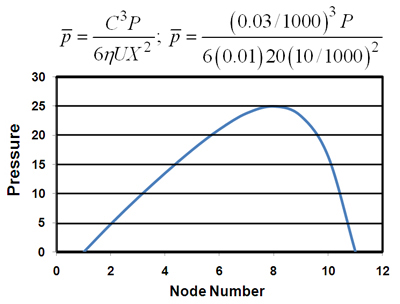
Fig. 5.17: Fluid pressure at various nodes.

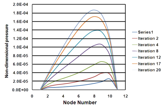
Fig. 5.18: Non-dimensional pressure over iteration.

Figures 5.17 and 5.18 illustrate variation in pressure profile. Pressure is minimum(ambient) at boundaries(nodes 1 and 11) and reaches to maximum at node 8(slightly away from mid-node).

The same example solved by numerical method in previous pages can be solved using long bearing approximation.

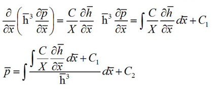
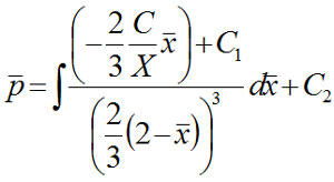
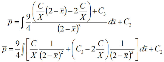
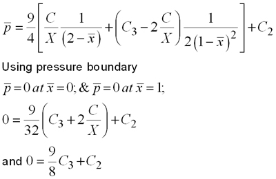
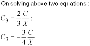
Generalized pressure expression for Approach1 :

For same film thickness expression().

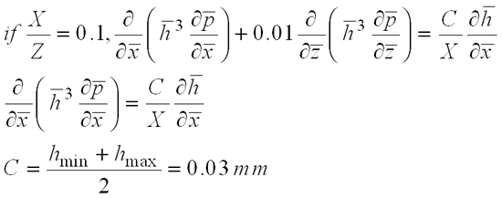
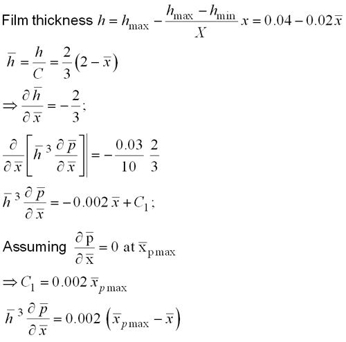
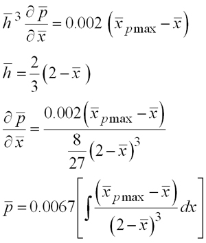
Example : Assume a thrust pad of 10*100 mm dimensions. Leading and trailing film thicknesses are 0.04 and 0.02 mm respectively. Sliding speed is 20 m/s. Viscosity of oil is 10 mPa.s and find pressure distribution.

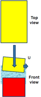
Fig. 5.19 : Thrust pad bearing.

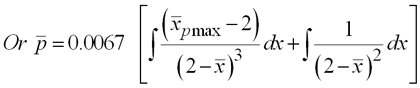
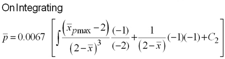
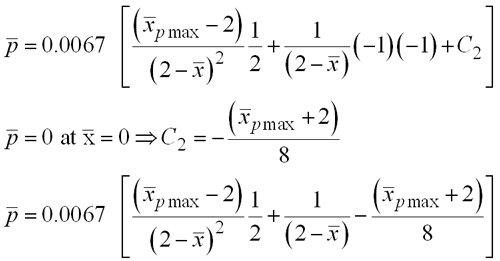
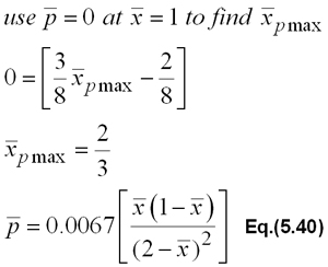
Using Eq.(5.40) non-dimensional pressure(Fig. 5.20) can be evaluated. We can compare this pressure with pressure calculated with numerical method(Fig. 5.21).

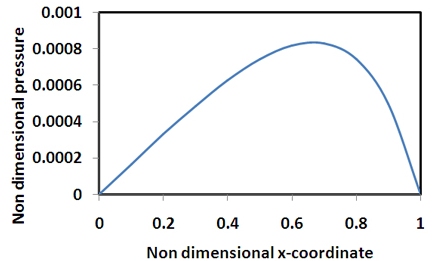
Fig. 5.20: Nondimensional pressure vs nondimensional x-coordinate.

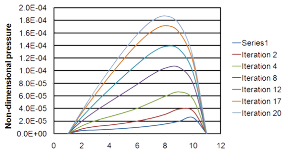
Fig. 5.21: Non-dimensional pressure calculated using numerical method.

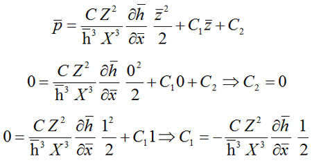
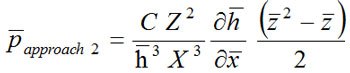
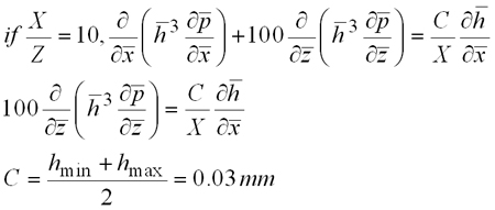
In second example we can consider short bearing (X/Z) = 10.

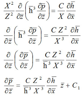
Generalized pressure expression for Approach2(short bearing approximation) :

Example : Assume a thrust pad of 100*10 mm dimensions. Leading and trailing film thicknesses are 0.04 and 0.02 mm respectively. Sliding speed is 20 m/s. Viscosity of oil is 10 mPa.s. Find pressure distribution.

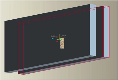
Fig. 5.22: Short bearing.

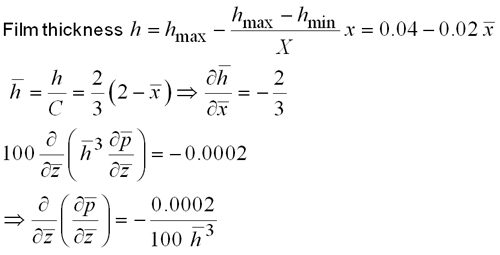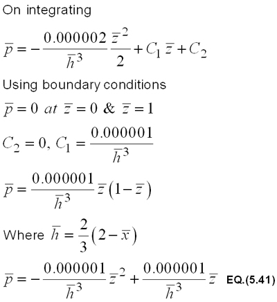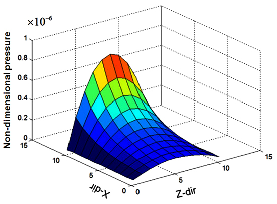
Fig. 5.23: Non-dimensional pressure using short bearing approximation.

Hybrid Solution Approach to solve Reynolds’ Equation

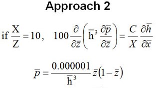
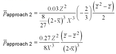
In previous part of the solving Reynolds’ equation, two approaches: long bearing approach (dimension in sliding direction much shorter than non-sliding direction: Approach 1) and short bearing approach ((dimension in sliding direction much larger than non-sliding direction: Approach 2) were considered. Both approaches are simple to implement and provide quick solution, but provide higher pressure values compared to actual fluid pressure developed by hydrodynamic actions. These approaches may provide reliable results in very short span of dimensions. To improve accuracy but maintain advantages of Approach 1/Approach2 we can hybridize these approaches. Two examples of extreme dimensions have been considered to illustrate the simplicity and accuracy of the hybrid approach. As hybrid approach requires pressure expressions obtain by Approach 1 and Approach 2, therefore derivation of fluid pressures have been detailed in the present heading.

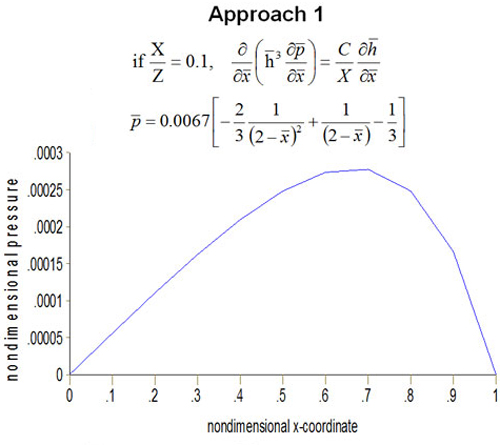
Fig. 5.24: Nondimensional pressure vs nondimensional x-coordinate.

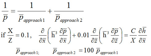
Hybridization :

This indicates that if dimension in sliding direction is relatively short, Approach 2 provides very INACCURATE pressure values.

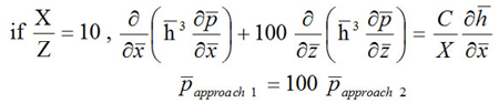This indicates that if dimension in sliding direction is relatively large, Approach 1 provides very INACCURATE pressure values.

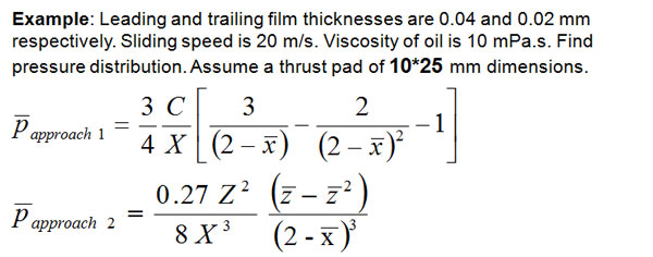
Example : Leading and trailing thicknesses are 0.04 and 0.02 mm respectively. sliding speed is 20 m/s. Viscosity of oil is 10 mPa.s. Find pressure distribution. In the present example

Let us consider two cases bearing dimensions for same film thickness expression. CASE 1 : Thrust pad of 100*10 mm dimensions.

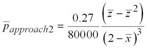....Eq.(5.42)

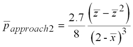....Eq.(5.43)

Case 1: Assume a thrust pad of 100 * 10 mm dimensions.

....Eq.(5.44)

Case 2: Assume a thrust pad of 10 * 100 mm dimensions.

....Eq.(5.45)

HYBRID APPROACH

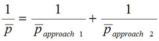CASE 1: Assume a thrust pad of 100 * 10 mm dimensions, use equations (5.42) and (5.44).

....Eq.(5.46)

CASE 2: Assume a thrust pad of 10 * 100 mm dimensions, use equations (5.43) and (5.45).

....Eq.(5.47)

Equations (5.46) and (5.47) are used to find pressure distribution for case 1 (Fig. 5.25a) and case 2 (Fig. 5.25b).

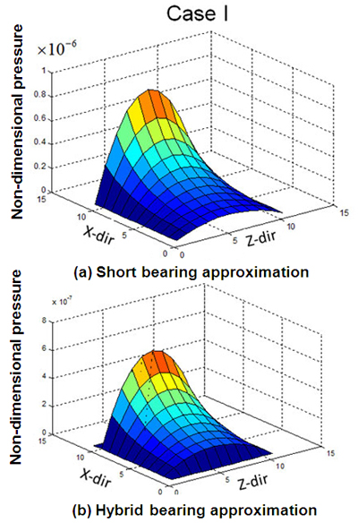
Fig. 5.25: Non-pressure calculated using short bearing and hybrid bearing approximation.

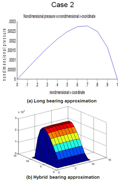
Fig. 5.26: Comparison between hybrid and Approach 1.

On studing Figures 5.25 and 5.26, it can be concluded that hybrid bearing approximation provides lesser value of fluid pressure compared to approaches 1 and 2. To get more confidence on hybrid approach let us consider following example :

Pressure expression does not change with value of Zin Approach 1. But pressure expression for approach 2 changes with change in dimensions either in X or Z direction.

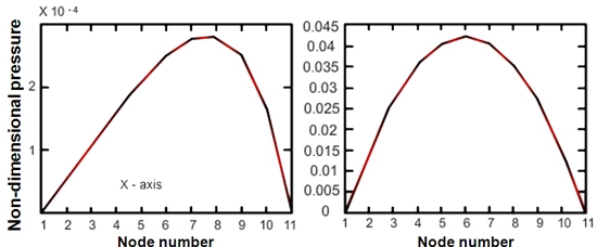
Fig. 5.27: Approach 1 ............................. Fig. 5.28: Approach 2.

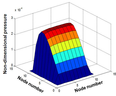
Fig. 5.29: Hybrid approach.

Non-dimensional pressure distribution obtained using Approach 1(long bearing), Approach 2(short bearing) and hybrid bearing are plotted in Figures 5.27 to 5.29 which plot provides better results can be judged based on results of finite difference method.

Finite Difference Method to solve Reynolds’ Equation

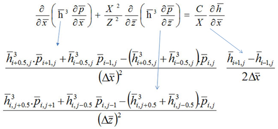
Finite Difference Method(By central difference method) :

After substitution and rearrangement.

....Eq.(5.48)

As pressures at i, j nodes are unknown(except boundary pressures), following approximation at 0th iteration is made

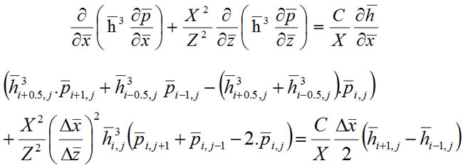
Assumption : film thickness only function of x :

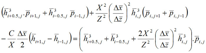
By simplification of above equation we get

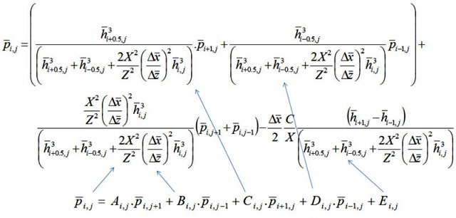
Non-dimensional nodal pressure :

We can remove subscript j from h terms and because we are taking equal spacing.

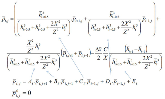We can make computer program to get pressure results.

Computer Program(Matlab program) :

N=50; % number of nodes in X-dir. M=50; % number of nodes in Z-dir. C = 0.030; % radial clearence in mm. Z1=25; % Length in axial direction(mm). X1 = 10; % Length in sliding direction. delxbar = 1/N; delzbar = 1/M; const1 = X1*X1/(Z1*Z1); ITER = 1000; % Number of iteration. for I=1:N+1 for J=1:M+1 p(I,J)=0.0; % Assigning zero pressure at every i, j node. end end sum(1)=0.0; for K = 1:ITER sumij=0.0; for I=2:N X(I)=1/N*(I-1); h=2/3*(2-X(I)); hm=2/3*(2-X(I)-0.5*delxbar); hp=2/3*(2-X(I)+0.5*delxbar); hm1=2/3*(2-X(I)-delxbar); hp1=2/3*(2-X(I)+delxbar); cubh=h*h*h; cubhm=hm*hm*hm; cubhp=hp*hp*hp; const2 = (cubhp+cubhm+2*const1*cubh); A=const1*cubh/const2; CA=cubhp/const2; D=cubhm/const2; E=-0.5*delxbar*(hp1-hm1)*C/(const2*X1); for J=2:M Z(J)=1/M*(J-1); p(I,J)=A*p(I,J+1)+A*p(I,J-1)+CA*p(I+1,J)+D*p(I-1,J)-E; sumij=sumij+p(I,J); end end sum(K+1)=sumij; percentage = abs(sum(K+1)-sum(K))/abs(sum(K+1)); if percentage < 0.0001 break end end y = K SURF(p); % Plot pressure in 3-D.

Effect of error(ε) on solution :

Error is evaluated using Eq.(5.39). Pressure distribution for error(ε) = 0.01 is shown in Fig. 5.30. Comparing pressure disribution shown in Fig. 5.31 with that in Fig. 5.30, it can be concluded that pressure is modified and the maximum pressure is slightly higher in Fig. 5.31. Pressure distribution shown in Fig. 5.31 and Fig. 5.32 are almost same which means convergence has occured.

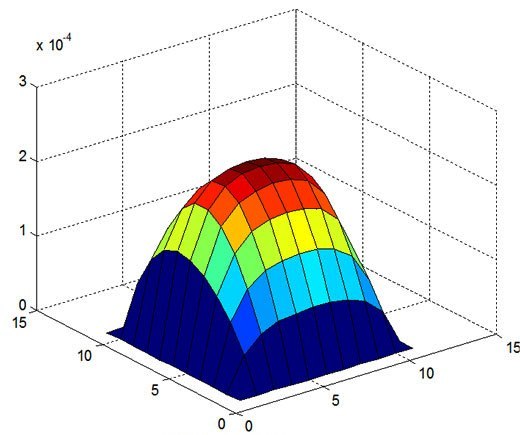
Fig. 5.30: Pressure distribution for ε = 0.01, N = 10, M = 10.

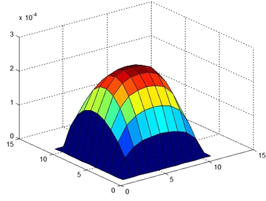
Fig. 5.31: Pressure distribution for ε = 0.001, N = 10, M = 10.

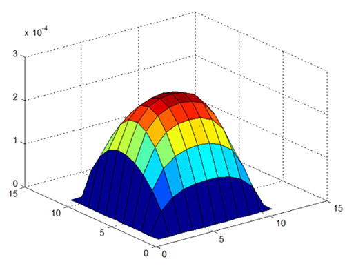
Fig. 5.32: Pressure distribution for ε = 0.0001, N = 10, M = 10.

Comparing results of pressure distributions obtained by Finite diffrence, hybrid approach and Approach 1. In previous subheading pressure distribution for thrust pad of 10 * 25 mm2 dimension was obtained using finite difference method. Pressure results are plotted in Fig. 5.33. On comparing Figures 5.33, 5.34 and 5.35 it can be said that pressure profile obtained by hybrid approach is very close to pressure profile obtained by FDM.

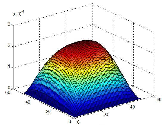
Fig. 5.33: Pressure distribution for ε = 0.001; Node 50 * 50, (X/Z) = 0.4.

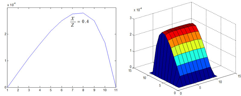
Fig. 5.34: Approach 1 ...................................... 5.35: Hybrid approach.

Conclusions :- 1. Hybrid approach provides better results compared to the results obtained by Approach 1 & Approach 2. 2. Accuracy of pressure results obtained by finite difference method (FDM) depends on the number of nodes (discretization of bearing space) and number of iterations. 3. To reduce the computation time required to estimate nodal pressures using FDM, we can assign initial pressure values obtained by hybrid approach and involving subsequent iteration using FDM.

Viscosity Variation

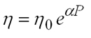
In deriving Reynolds equation in previous subheading, an assumption of constant viscosity was made. In practice viscosity is function of pressure and it increases with increase in fluid pressure, as given in Eq.(5.49).

Eq.(5.49)

On substituting this viscosity relation in static Reynolds equation.

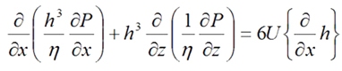....Eq.(5.50)

....Eq.(5.51)

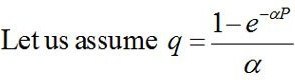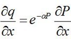....Eq.(5.52)

Using Eq.(5.52) in Eq.(5.51), we get

....Eq.(5.53)

This Reynolds’ equation does not consider the shape of the surfaces under high pressure. It only encompasses the alteration in the viscosity by defining reduced pressure. For multigrade oils, viscosity is represented as :

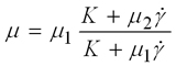....Eq.5.53(c)

Using Eq 5.53(c), Reynolds equation for multigrade oil is presented as:

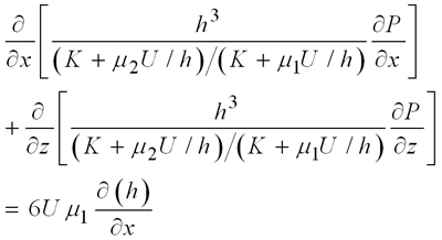Eq.5.53(d)

Effect of pressure viscosity relation :

Pressure profilies obtained by using Eq.(5.50) and Eq.(5.53) after converting reduce pressure to fluid pressure have been plotted in Fig. 5.36 and Fig. 5.37 respectively. No noticeable difference in pressures is observed. In other words for low viscosity oil, pressure viscosity does not bring much difference in pressure.

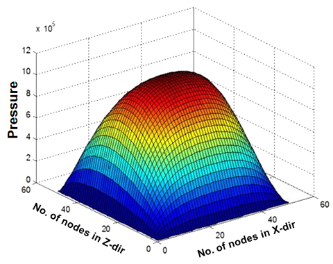
Fig. 5.36: Pressure distribution without pressure viscosity, relation viscosity = 10 mPa.s

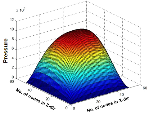
Fig. 5.37: Pressure distribution with pressure viscosity relation

Effect of pressure viscosity relation for thicker oils :

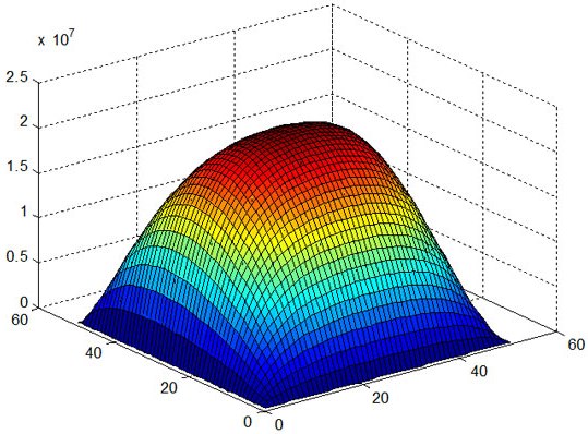
Fig. 5.38: Pressure distribution without pressure viscosity relation, viscosity = 200 mPa.s

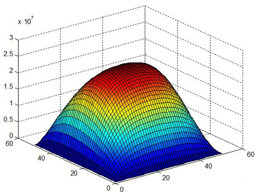
Fig. 5.39: Pressure distribution with pressure viscosity relation, viscosity 200mPa.s

On comparing Figures 5.38 and 5.39, an increase in fluid pressure on accounting pressure viscosity relation is observed.

Effect of pressure viscosity relation on increasing relative velocity :

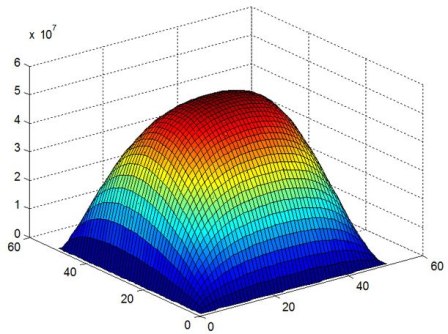
Fig. 5.40: Pressure distribution without pressure viscosity relation (200mPa.s, V = 50 m/s)

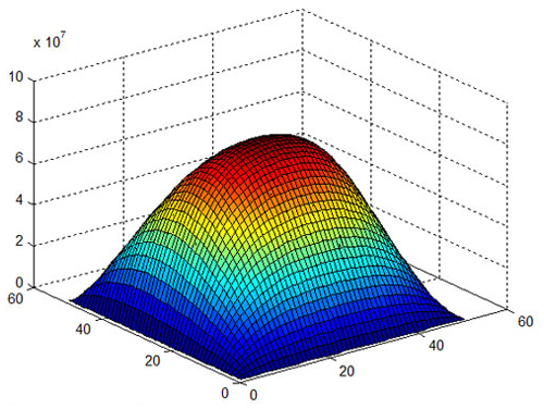
Fig. 5.41: Pressure distribution with pressure viscosity relation, viscosity 200mPa.s, V = 50 m/s.

VISCOSITY Temperature Relationship :

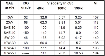
Lubricant viscosity is a strong function of temperature, as illustrated in Table 5.3. Vogel and Wather’s relations are often used to express dependence of viscosity on temperature. • Vogel`s equation : η = keb/(t + θ). k gives inherent viscosity. b has unit of temperature. b increases with increase in viscosity. • Walther`s Equation loglog(cS + 0.6) = constant - c log T.

Table 5.3: Variation in viscosity with temperature.

Using these equations (Vogel/Walther) effect of temperature on pressure can be evaluated.

Reynolds equation for compressible fuid. On accounting density variation of fluid Reynolds equation is given by

....Eq.5.53(a)

First two terms of this equation represent pressure-flow in two directions (in the plane of rotation). Maximum complexity of Reynolds equation lies in these two terms, due to : • Relation between density ρ and pressure P in aero- dynamic/static lubrication. • Relation between viscosity, μ and pressure P; and relation between film thickness h and pressure P in elasto hydrodynamic lubrication. • Relation between viscosity μ and film thickness for multigrade liquids. • Relation between viscosity μ and temperature (that depends on pressure) for thermal analysis. As viscosity of gases is almost independent of temperature and pressure, Reynolds equation Eq 5.53(a) for aerodynamic lubrication is presented as :

....Eq.5.53(b)

Importance of viscosity : Streibeck curve shows how the viscosity of lubricant affects the nature and quality of the lubrication. Somerfield number on x-axis depends on viscosity, relative speed and mean pressure (specific load). If load and speed are constant. Viscosity divides lubrication in three zones. Zone 3 : Complete separation, thick film, hydrodynamic lubrication. Friction is entirely viscous friction caused by mechanical shearing. Point C just sufficient to ensure complete separation of surfaces. Point C ideal point to provide zero wear with almost minimum friction. Zone2 : Load is carried partly by the film of lubricant and partly by asperity interaction. Zone 1 : Zone of boundary lubrication. Chemical and physical properties of lubricant other than its bulk viscosity control the quality of lubrication.

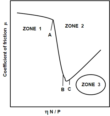
Fig. 5.42(a): Stribeck curve.

Petroff’s Equation :

To account thermal effects, we need to calculate friction loss. Petroff’s equation provides crude estimation of friction loss in sliding bearing.

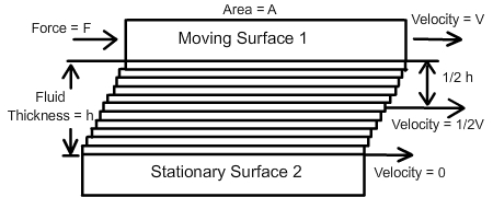
Fig. 5.42(b): Lubricant shearing.

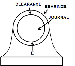
Fig. 5.43: Sliding bearing.

Petroff assumed concentric position of shaft as shown in Fig. 5.43. To derive friction he assumed shearing(Fig. 5.42(b)) of Newtonian lubricant.

Friction = Shear stress * Area F = (Viscosity * V/h) * Area V = 2πRN; A = 2πRL F = (η * 2πRN * 2πRL)/C....Eq.(5.54) C is radial clearence. Equation(5.54) is known as Petroff`s equation. This equation can be used to estimate generated heat. Heat generated H = F.V ....Eq.(5.55)

Temperature Rise :

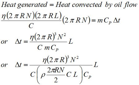
Friction, due to shear of lubricant film, generates heat (F * V) in lubricant oil(Eq. 5.55) and increases the temperature of lubricant. Assuming that total generated heat is carried by the oil flowing through bearing.

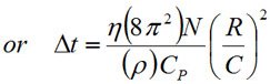....Eq.(5.56)

Assume ρ = 860 kg/m3 CP = 1760 J/(Kg0C) R/C = 1000 η = ηin e-β(t - tin) After substitution Δt = 52.2 η N....Eq.(5.57)

Assume rotational speed = 900 rpm. Δt = 783 η....Eq.(5.58) In hydrodynamic lubrication, increase in viscosity increases load capacity but also increases friction and temperature(Eq. 5.58), therefore careful selection of viscosity is important.

Elastic Deformation

In previous paragraphs effect of pressure on viscosity was considered. In the present heading, we shall consider effect of pressure on elasticity of the contacting (or non-contacting) materials. It is generally known that elastic deformation of the material depends on “Young’s modulus” and “Poisson’s ratio”. Under compressive load, elastic deformation of surfaces over a region surrounding the initial point of contact occurs, as shown in Fig. (5.45). Associated stresses are highly dependent on geometry of the surfaces in contact as well as loading and material properties.

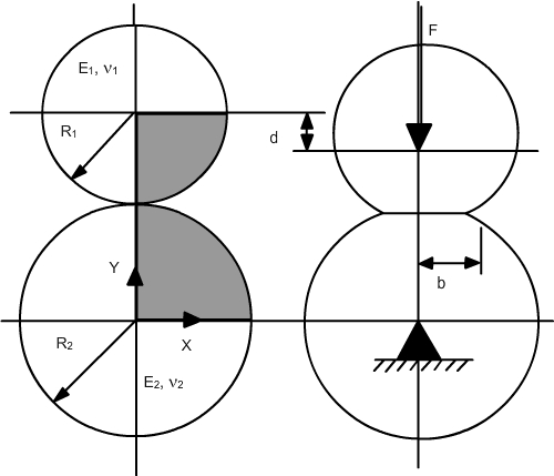
Fig. 5.44: Spherical objects in without contact load...........Fig. 5.45: Spherical objects in contact under compressive load.

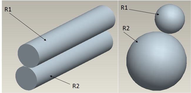
Fig. 5.46: Cylindrical objects in contact. ...................... Fig. 5.47: Spherical objects in contact.

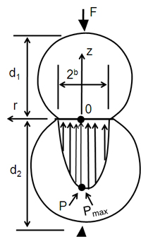
Fig. 5.48: Pressure profile.

Elasto-hydrodynamic lubrication

Due to elastic deformation caused by compressive loading, a flat surface is created(as shown in Fig. 5.48) which allows lubricant to be captured. Such mechanism, known as elasto-hydrodynamic lubrication, increases the load capacity of hydrodynamic action.

Spherical contact :

Pressure distribution in EHL between spherical(Fig. 5.48) object can modeled using.

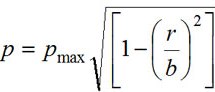....Eq.(5.59)

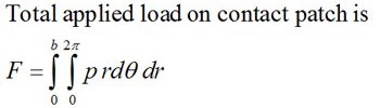
Here Pmax is the max, fluid pressure, 2b is total contact patch perpendicular to normal load r varies between zero to value b.

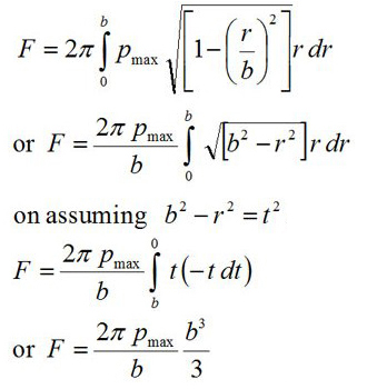
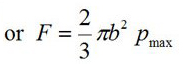
On substituting expression of p from Eq.(5.59).

....Eq.(5.60)

Cylindrical Contact :

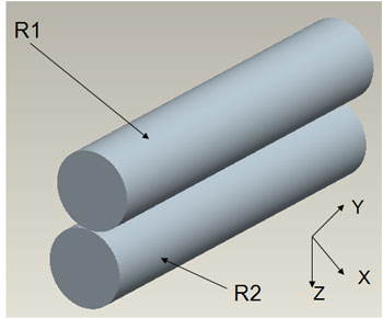
Fig. 5.49: Cylindrical contact.

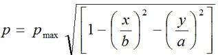
Pressure distribution in cylindrical contact can be given by Eq.(5.61).

....Eq.(5.61)

Pressure variation along Y - axis is negligible, Therefore

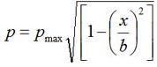....Eq.(5.62)

Total applied load on contact patch can be obtained by substituting Eq.(5.62) and integrating over cylindrical length.

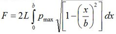Let x = b sin θ. Total applied load on contact patch is

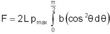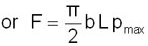....Eq.(5.63)

On comparing 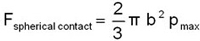with 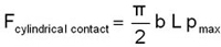it can be said that F in cylindrical contact > F in spherical contact.

Elastic Deformation suggested by Timoshenko & Goodier :

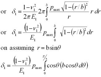
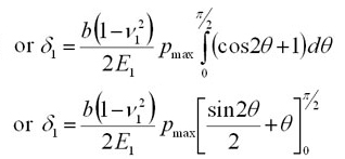
Equation(5.60) and (5.63) requires expression of b to estimate the load capacity. To find b we can use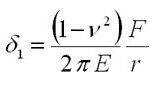

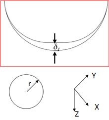
Fig. 5.50: Elastic deformation in Z-dir under compressive load.

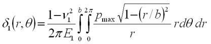....Eq.(5.64)

....Eq.(5.65)

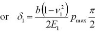
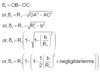
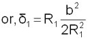
Deflection δ1 can be approximate using Fig. (5.51).

....Eq.(5.66)

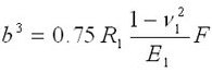
On using Equations (5.65), (5.66) and (5.60); and rearranging

....Eq.(5.67)

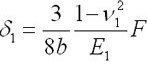....Eq.(5.68)

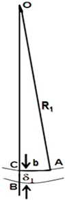
Fig. 5.51: Sketch to express δ1.

How to incorporate deflection in FDM :

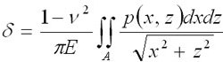
In previous paragraphs we derived analytical expression of deflection, but for generic geometry we need to use numerical methods, i.e., FDM, FEM.

....Eq.(5.69)

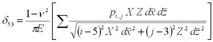
In FDM, nodal pressure Pi,j are evaluated which can be incorporated in Eq.(5.69).

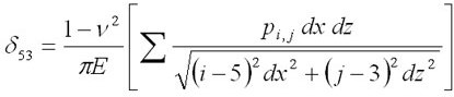Deflection at each node needs to be evaluated.

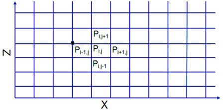
Fig. 5.52: Grid arrangement for FDM.

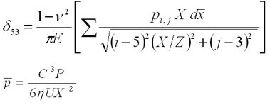
On non-dimensionlizing

Or.. ....Eq.(5.70)

Finite Difference Method :

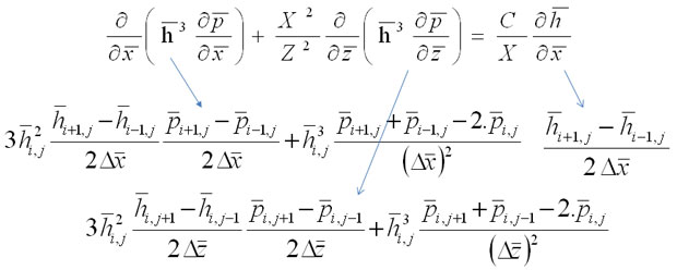
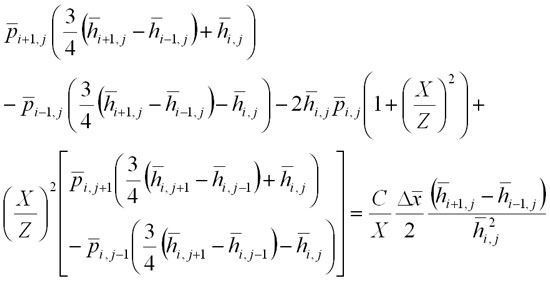
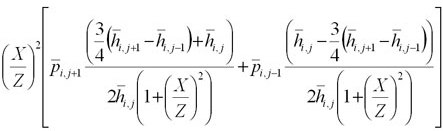
In EHL we need to combine hydrodynamic and elastic deformation. To integrate both the action we can solve Reynolds equation and update film thickness by incorporating local elastic deformation.

Or

....Eq.(5.71)

Eq.(5.71) can be solved using iteration and for each evaluated nodal pressure film thickness can be updated by incorporating Eq.(5.70). Fig.(5.53) shows pressure profiles for same geometric dimension.

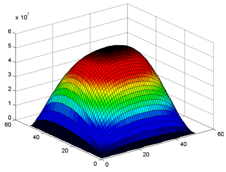
Fig. 5.53(a): Pressure profile accounting only hydrodynamic action.

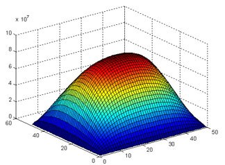
Fig. 5.53(b): Pressure profile accounting viscosity pressure relation.

Deflection curve :

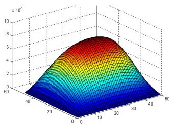
Fig. 5.53(c): Pressure profile accounting viscosity pressure and elastic deformation in hydrodynamic action.

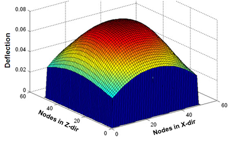
Fig. 5.54: Deflection curve.

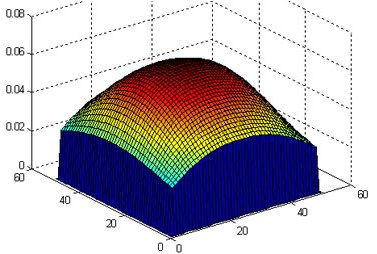
Fig. 5.55: Deflection curve after accounting elastic deformation

Om comparing figures 5.54 and 5.55, lesser deflection in Fig. (5.55) is observed. This means modification in film thickness, reduces local deformation.

Pressure distribution :

Due to elastic deformation, maximum value of pressure decreases and more uniform pressure distribution occurs as shown in Fig. 5.56.

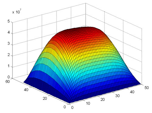
Fig. 5.56: Pressure distribution accounting EHL.

Thermo-hydrodynamic lubrication

In previous paragraphs elastohydrodynamic lubrication mechanism was explained. In the present subheading we are going to discuss thermo-hydrodynamic lubrication. The analysis of a hydrodynamic lubrication problem with allowance for viscous heating is commonly known as thermohydrodynamics.

Why should we consider thermal heating ?

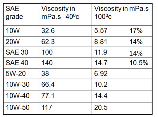
Answer of this question is provided in Table (5.4) which lists significant reduction in fluid viscosity on increasing temperature occurs, which may reduce load carrying capacity.

Table 5.4

How to account Thermal effects ?

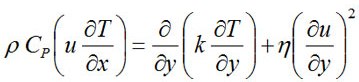
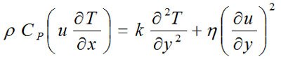
We need to solve energy equation with hydrodynamic equation(Eq. 5.72) Energy Equation: The energy equation is a simplified form of the heat transfer equation commonly used in fluid mechanics.

....Eq.(5.72)

In the present case Φ = τ(δu/δy) For Newtonian fluid Φ = η(δu/δy)2 where • u lubricant velocity in the direction of sliding [m/s]; • p lubricant density [kg/m3]; • Cp is the specific heat of the lubricant [J/kg K]; • K is the thermal conductivity of the lubricant [W/mK]; • w is the lubricant velocity in the ‘z’ direction [m/s]; • x is the co-ordinate in the direction of sliding [m]; • y is the co-ordinate normal to the horizontal plane of the lubricant film [m].

Terms present in the heat transfer equation can be eliminated by an order of magnitude analysis to yield only the convection terms and the conduction normal to the plane of the film. The characteristics of pressure and shear stress equilibrium in the oil film are unchanged except that the viscosity is variable in all three dimensions, i.e. viscosity also varies through the film thickness.

Simplified Energy Equation :

Or

Or

....Eq.(5.73)

Or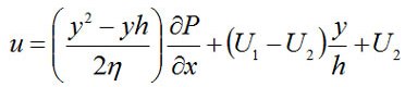

where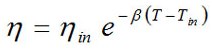

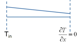
Fig. 5.57: Boundary condition.

To solve Eq.(5.73) we require boundary conditions. Temperatures at the outlet are unknown and can be calculated by applying the boundary condition ∂/∂x = 0(Fig. 5.57). The condition ∂T/∂x = 0 relates to the very slow change in temperature by cooling once the lubricant leaves the bearing exit.