Section IV:    Long Line Model

For accurate modeling of the transmission line we must not assume that the parameters are lumped but are distributed throughout line. The single-line diagram of a long transmission line is shown in Fig. 2.5. The length of the line is l . Let us consider a small strip Δx that is at a distance x from the receiving end. The voltage and current at the end of the strip are V and I respectively and the beginning of the strip are V + ΔV and I + Δ I respectively. The voltage drop across the strip is then ΔV . Since the length of the strip is Δx , the series impedance and shunt admittance are z Δx and y Δx . It is to be noted here that the total impedance and admittance of the line are

(2.24)

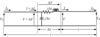
Fig. 2.5 Long transmission line representation.

From the circuit of Fig. 2.5 we see that

(2.25)

Again as Dx ® 0, from (2.25) we get

(2.26)

Now for the current through the strip, applying KCL we get

(2.27)

The second term of the above equation is the product of two small quantities and therefore can be neglected. For Dx ® 0 we then have

(2.28)

Taking derivative with respect to x of both sides of (2.26) we get

Substitution of (2.28) in the above equation results

(2.29)

The roots of the above equation are located at ±√( yz ). Hence the solution of (2.29) is of the form

(2.30)

Taking derivative of (2.30) with respect to x we get

(2.31)

Combining (2.26) with (2.31) we have

(2.32)

Let us define the following two quantities

	(2.33)
	(2.34)

Then (2.30) and (2.32) can be written in terms of the characteristic impedance and propagation constant as

	(2.35)
	(2.36)

Let us assume that x = 0. Then V = V_R and I = I_R . From (2.35) and (2.36) we then get

	(2.37)
	(2.38)

Solving (2.37) and (2.38) we get the following values for A₁ and A₂ .

Also note that for x = l we have V = V_s and I = I_S . Therefore replacing x by l and substituting the values of A₁ and A₂ in (2.35) and (2.36) we get

	(2.39)
	(2.40)

Noting that

We can rewrite (2.39) and (2.40) as

	(2.41)
	(2.42)

The ABCD parameters of the long transmission line can then be written as

	(2.43)
	(2.44)
	(2.45)