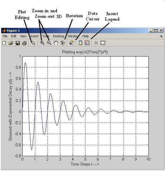
MATLAB MODULE 1MATLAB Window Environment and the Base Program PlottingMATLAB is an outstanding tool for visualization. In the following, we will learn how to create and print simple plots. We are going to plot sinusoidal oscillations with exponential decay. To do this, first generate the data ( x- and y- coordinates). x- coordinate in this case is time steps. Let the initial time >> t=0:0.05:10; % Generating time steps >> yt=exp(-t/2).*sin(2*pi*t); %Calculate y(t ) >> plot(t,yt); %Plot t vs. y(t ) >> grid on; %Generating grids on x- and y-coordinates >> xlabel('Time Steps: t --->'); %Labeling x-axis >> ylabel('Sinusoid with exponential decay: y(t) --->'); %Labeling y-axis >> title('Plotting exp(-t/2)*sin(2*pi*t)'); %Put a title on the plot
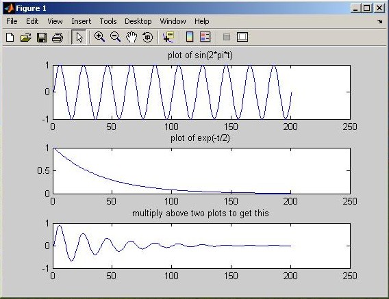
Response is shown in graphics or figure window snapshot (Fig. M1.15). Arguments of the xlabel, ylabel, and title commands are text strings. Text strings are entered within single-quote characters. Lines beginning with % are comments; these lines are not executed. The print command sends the current plot to the printer connected to your computer. Rather than displaying the graph as a continuous curve, one can show the unconnected data points. To display the data points with small stars, use plot(t,yt,'*'). To show the line through the data points in red color as well as the distinct data points, one can combine the two plots with the command plot(t,yt,'r',t,yt,'*'). To learn more about plot options, type help plot on the MATLAB prompt and hit return. One can also produce multiple plots in a single window. Enter the following sequence of commands to your MATLAB command window and observe the resultant figure (Fig. M1.16).
Fig. M1.15 Plotting sinusoid with exponential decay
>> subplot(3,1,1);plot(sin(2*pi*t)); >> title('plot of sin(2*pi*t)'); >> subplot(3,1,2);plot(exp(-t/2)); >> title('plot of exp(-t/2)'); >> subplot(3,1,3);plot(exp(-t/2).*sin(2*pi*t)); >> title('multiply above two plots to get this');
Fig. M1.16 Plotting multiple plots in a single figure window
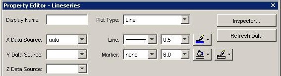
The command subplot(m,n,p) breaks the figure window into an m-by-n matrix of small axes and selects the pth axes for the current plot. Labeling, title, and grid commands should be given immediately after the particular subplot command to apply them to that subplot. Learn more about subplot using help subplot . Click on the Plot Editor icon Double clicking anywhere exactly on the curve opens the Property Editor � Lineseries (Fig M1.18). From this, plot type can be changed on the spot. Available plot options are: Line, Area, Bar, Stairs, and Stem. Line width and markers can be changed by pull down menu Line and Marker.
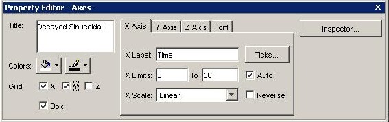
Fig. M1.17 Axes property editor
Fig. M1.18 Lineseries property editor
|
 for:
for:  for t = [0:0.1:10].
  . Using MATLAB, generate the following two plots on semilog graph sheet for