If you know the exact name of a command, type help
commandname to get detailed task-oriented help. For example, type
help helpwin in the command window to get the help on the command
helpwin .
If you don't know the exact command, but (atleast !) know the keyword related to the task you want to perform, the
lookfor command may assist you in tracking the exact command. The
help command searches for an exact command name matching the keyword, whereas the
lookfor command searches for quick summary information in each command related to the keyword. For example, suppose that you were looking for a command to take the inverse of a matrix. MATLAB does not have a command named
inverse; so the command
help inverse will not work. In your MATLAB command window try typing
lookfor inverse to see the various commands available for the keyword
inverse.
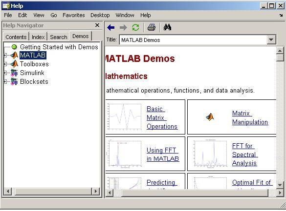
MATLAB has a wonderful demonstration program that shows its various features through interactive graphical user interface. Type
demo at the MATLAB prompt to invoke the demonstration program (Fig. M1.14) and the program will guide you throughout the tutorials.
Elementary Matrices
Basic data element of MATLAB is a matrix that does not require dimensioning. To create the matrix variable in MATLAB workspace, type the statement (note that any operation that assigns a value to a variable, creates the variable, or overwrites its current value if it already exists).
>> A=[8 1 6 2;3 5 7 4;4 9 2 6] 
The blank spaces (or commas) around the elements of the matrix rows separate the elements. Semicolons separate the rows. For the above statement, MATLAB responds with the display
A =
8 1 6 2
3 5 7 4
4 9 2 6
Vectors are special class of matrices with a single row or column. To create a column vector variable in MATLAB workspace, type the statement
>> b=[1; 1; 2; 3] 
b =
1
1
2
3
To enter a row vector, separate the elements by a space or comma ' , '. For example:
>> b=[1,1,2,3] 
b =
1 1 2 3
We can determine the size of the matrices (number of rows, number of columns) by using the size command.
>> size(A) 
ans =
3 4
The command size, when used with the scalar option, returns the length of the dimension specified by the scalar. For example,
size (A,1) returns the number of rows of
A and size(A,2)
returns the number of columns of A.
>> size(A,1) 
ans =
3
>> size(A,2) 
ans =
4
For matrices, the length command returns either number of rows or number of columns, whichever is larger. For example,
>> length(A) 
ans =
4
For vectors, length command can be used to determine its number of elements.
>> length(b) 
ans =
4
The use of colon ( : ) operator plays an important role in MATLAB. This operator may be used to generate a row vector containing the numbers from a given starting value
xi, to the final value
xf, with a specified increment
dx, e.g., x=[xi:dx:xf]
>> x=[0:0.1:1] 
x =
Columns 1 through 7
0 0.1000 0.2000 0.3000 0.4000 0.5000 0.6000
Columns 8 through 11
0.7000 0.8000 0.9000 1.0000
By default, the increment is taken as unity.
To generate linearly equally spaced samples between x1 and x2, use the command
linspace(x1,x2) . By default, 100 samples will be generated. The command
linspace (x1,x2, N) allows the control over number of samples to be generated. See the example below.
>> x=linspace(0,1,11)
x =
Columns 1 through 6
0 0.1000 0.2000 0.3000 0.4000 0.5000
Columns 7 through 11
0.6000 0.7000 0.8000 0.9000 1.0000
Learn how to generate logarithmically spaced vector using the command
logspace .
The colon operator can also be used to subscript matrices. For example,
A(:,j) is the jth column of
A, and
A(i,:) is the ith row of
A. Observe the following MATLAB session.
>> A=[8 1 6 2;3 5 7 4;4 9 2 6]; 
>> A(2,:) 
ans =
3 5 7 4
>> A(3,2:4) 
ans =
9 2 6
>> A(1,3) 
ans =
6
>> B=A(1:3,2:3) 
B =
1 6
5 7
9 2
>> A(:,3)=[ ] 
A =
8 1 2
3 5 4
4 9 6
Manipulating matrices is almost as easy as creating them. Try the following operations:
>> A+3 
>> A-3 
>> A*3 
>> A/3 
When you add/subtract/multiply/divide a vector/matrix by a number (or by a variable with a number assigned to it), MATLAB assumes that all elements of vector/matrix should be individually operated on.
Table M1.3 provides the list of basic operations on any two arbitrary matrices A and B and their dimensional requirements.
Example M1.1
To find the solution of the following set of linear equations:
we write the equations in the matrix form as

where
 is the matrix of coefficients of x1, x2 and x3
 is the column vector which will contain the solutions x1, x2 and x3
 is the column vector of values on the right-hand side
The solution vector
where stands for adjoint of matrix and
  stands for determinant of
The determinant of  matrix
is a scalar-valued function of . It is found through the use of minors and cofactors.
The minor mij of the element aij is the determinant of a matrix of order  obtained from by removing the row and column containing aij. The cofactor cij of the element aij is defined by the equation
Determinants can be evaluated by an expansion that reduces the evaluation of an  determinant down to the evaluation of a string of determinants, namely the cofactors. Selecting an arbitrary row k of matrix or arbitrary column l of matrix , we have
or

The adjoint of  matrix is found by replacing each element aij of matrix by its cofactor and then transposing.
Following MATLAB commands solve the given set of simultaneous linear equations.
>> A = [2 5 -3; 3 -2 4; 1 6 -4];
>> b = [6; -2; 3];
>> x = inv(A) * b
x =
4.8333
-4.5833
-6.4167
 .
.