MATLAB MODULE 1MATLAB Window Environment and the Base Program Starting MATLABOn the Windows desktop, the installer usually creates a shortcut icon for starting MATLAB; double-clicking on this icon opens MATLAB desktop.
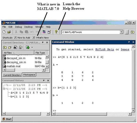
The MATLAB desktop is an integrated development environment for working with MATLAB suite of toolboxes, directories, and programs. We see in Fig. M1.1 that there are four panels, which represent:
A particular window can be activated by clicking anywhere inside its borders.
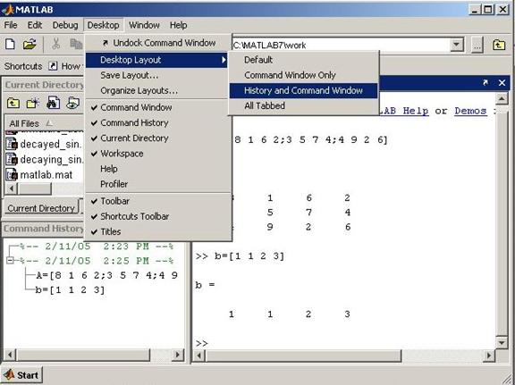
Fig. M1.1 MATLAB Desktop (version 7.0, release 14) Desktop layout can be changed by following Desktop --> Desktop Layout from the main menu as shown in Fig. M1.2 (Default option gives Fig. M1.1).
Fig. M1.2 Changing Desktop Layout to History and Command Window option
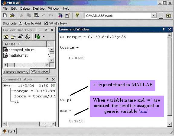
Command Window We type all our commands in this window at the prompt ( >> ) and press return Working with Command Window allows the user to use MATLAB as a versatile scientific calculator for doing online quick computing. Input information to be processed by the MATLAB commands can be entered in the form of numbers and arrays. As an example of a simple interactive calculation, suppose that you want to calculate the torque ( T ) acting on 0.1 kg mass ( m ) at >> torque = 0.1*9.8*0.2*pi/6 MATLAB responds to this command by: torque = 0.1026 MATLAB calculates and stores the answer in a variable torque (in fact, a
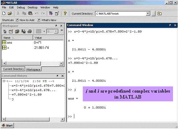
Fig. M1.3 Command Window for quick scientific calculations ( text in colored boxes corresponds to explanatory notes ). If any statement is followed by a semicolon, >> m = 0.1; >> l = 0.2; >> g = 9.8; the display of the result is suppressed. The assignment of the variable has been carried out even though the display is suppressed by the semicolon. To view the assignment of a variable, simply type the variable name and hit Enter. For example: >> torque=m*g*l*pi/6; >> torque torque = 0.1026 It is often the case that your MATLAB sessions will include intermediate calculations whose display is of little interest. Output display management has the added benefit of increasing the execution speed of the calculations, since displaying screen output takes time. Variable names begin with a letter and are followed by any number of letters or numbers (including underscore). Keep the name length to 31 characters, since MATLAB remembers only the first 31 characters. Generally we do not use extremely long variable names even though they may be legal MATLAB names. Since MATLAB is case sensitive, the variables A and a are different. When a statement being entered is too long for one line, use three periods, � , followed by >> x=3-4*j+10/pi+5.678+7.890+2^2-1.89 >> x=3-4*j+10/pi+5.678... +7.890+2^2-1.89 + addition, The basic MATLAB trigonometric commands are sin, cos, tan, cot, sec and csc. The inverses Variables j =
Fig. M1.4 Command Window with example operations
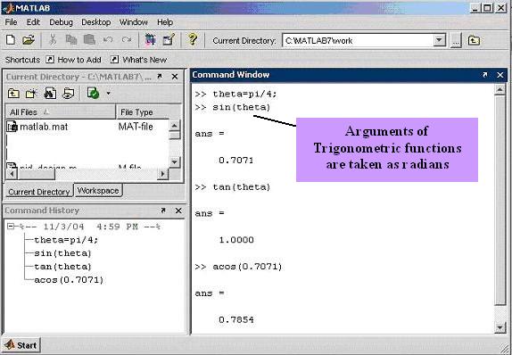
Fig. M1.5 Example trigonometric calculations
MATLAB representation of complex number
The later case is always interpreted as a complex number, whereas, the former case is a complex number in MATLAB only if j has not been assigned any prior local value. MATLAB representation of complex number
In Cartesian form, arithmetic additions on complex numbers are as simple as with real numbers. Consider two complex numbers
For example, two complex numbers >> z1=3+4j; >> z2=1.8+2j; >> z=z1+z2 z = 4.8000 + 6.0000i Multiplication of two or more complex numbers is easier in polar/complex exponential form. Two complex numbers with radial lengths
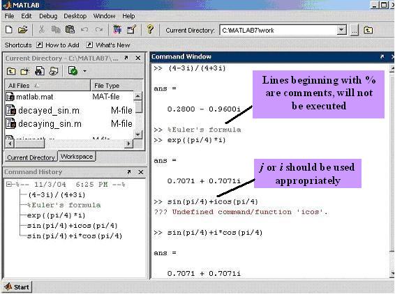
This can be done in MATLAB by: >> theta1=(35/180)*pi; >> z1=2*exp(theta1*j); >> z2=2.5*exp(0.25*pi*j); >> z=z1*z2 z = 0.8682 - 4.9240j Magnitude and phase of a complex number can be calculated in MATLAB by commands abs and angle. The following MATLAB session shows the magnitude and phase calculation of complex numbers >> abs(5*exp(0.19*pi*j)) ans = 5 >> angle(5*exp(0.19*pi*j)) ans = 0.5969 >> abs(1/(2+sqrt(3)*j)) ans = 0.3780 >> angle(1/(2+sqrt(3)*j)) ans = -0.7137 Some complex numbered calculations are shown in Fig. M1.6.
Fig. M1.6 Example complex numbered calculations
The mathematical quantities All computations in MATLAB are performed in double precision . The screen output can be displayed in several formats. The default output format contains four digits past the decimal point for nonintegers. This can be changed by using the format command. Remember that the format command affects only how numbers are displayed, not how MATLAB computes or saves them. See how MATLAB prints
The following exercise will enable the readers to quickly write various mathematical formulas, interpreting error messages, and syntax related issues.
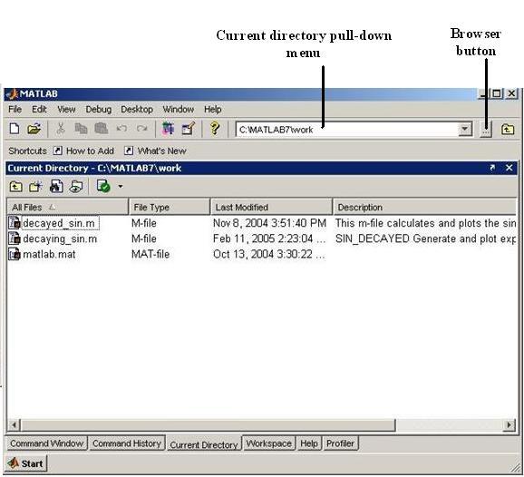
Current Directory Window This window (Fig. M1.7) shows the directory, and files within the directory which are in use currently in MATLAB session to run or save our program or data. The default directory is �C:\MATLAB7\work'. We can change this directory to the desired one by clicking on the square browser button near the pull-down window.
Fig. M1.7 Current directory window
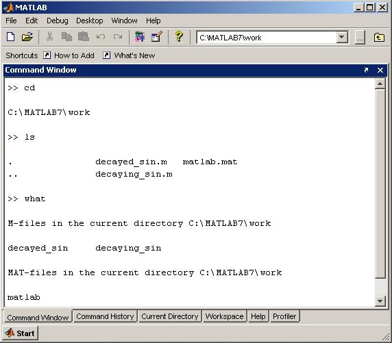
One can also use command line options to deal with directory and file related issues. Some useful commands are shown in Table M1.1.
Table M1.1
MATLAB desktop snapshot showing selected commands from Table M1.1 are shown in Fig. M1.8.
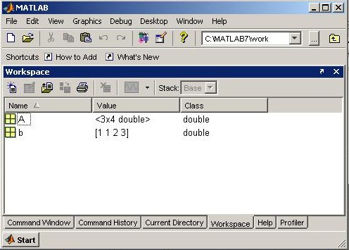
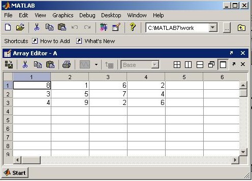
WorkspaceWorkspace window shows the name, size, bytes occupied, and class of any variable defined in the MATLAB environment. For example in Fig.M1.9, �b' is 1 X 4 size array of data type double and thus occupies 32 bytes of memory. Double-clicking on the name of the variable opens the array editor (Fig. M1.10). We can change the format of the data (e.g., from integer to floating point), size of the array (for example, for variable A, from 3 X 4 array to 4 X 4 array) and can also modify the contents of the array.
Fig. M1.8 Example directory related commands
If we right-click on the name of a variable, a menu pops up, which shows various operations for the selected variable, such as: open the array editor, save selected variable for future usage, copy, duplicate, and delete the variable, rename the variable, editing the variable, and various plotting options for the selected variable.
Fig. M1.9 Entries in the Workspace
Fig. M1.10 Array editor window Workspace related commands are listed in Table M1.2. Table M1.2
For example, see the following MATLAB session for the use of who and whos commands. >> who Your variables are: A b >> whos
Grand total is 16 elements using 128 bytes
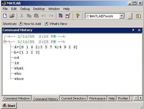
Command History Window This window (Fig. M1.11) contains a record of all the commands that we type in the command window. By double-clicking on any command, we can execute it again. It stores commands from one MATLAB session to another, hierarchically arranged in date and time. Commands remain in the list until they are deleted.
Fig. M1.11 Command history window
Commands can also be recalled with the up-arrow Selecting one or more commands and right-clicking them, pops up a menu, allowing users to perform various operations such as copy, evaluate, or delete, on the selected set of commands. For example, two commands are being deleted in Fig. M1.12.
|
 .
.  .
.