MATLAB MODULE 7Root Locus Design and SISO Design Tools
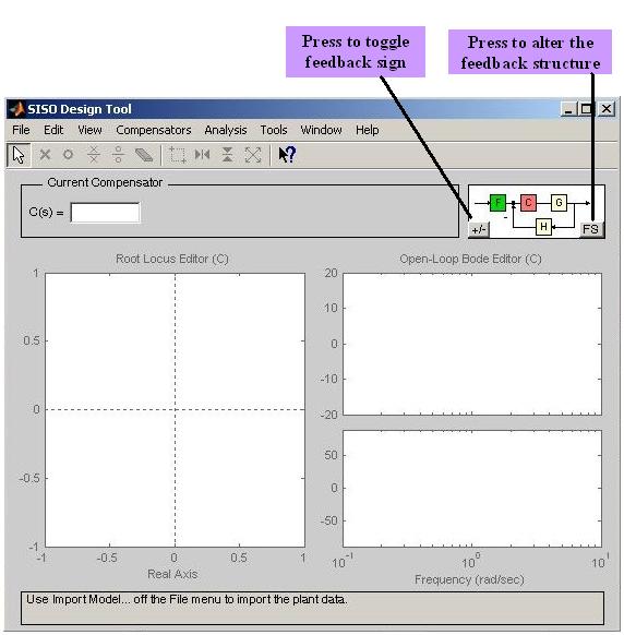
MATLAB's SISO Design Tool The SISO ( Single- Input/ Single- Output) Design Tool is a graphical user interface which allows one to design single-input/single-output compensators by interacting with the root locus plots and Bode plots of the closed-loop/open-loop systems. The tool also has the option of using a Nichols chart, which can be selected under the View menu. After the tool produces these plots, one can adjust the closed-loop poles along the root locus and read gain, damping ratio, natural frequency, and pole locations. These changes immediately get reflected to Bode plots and immediate changes in the system's closed-loop response can be viewed in the LTI Viewer for SISO Design Tool window. One can add poles, zeros, and compensators, which can be interactively changed to see the immediate effects on the root locus, Bode plots, and time response. With Bode plots, one can affect the gain change by shifting the Bode magnitude curve up and down; and gain, gain margin, gain crossover frequency, phase margin, phase crossover frequency, and whether the loop is stable or unstable can be checked. These changes immediately get reflected to root locus plots and immediate changes in the system's closed-loop response can be viewed in the LTI Viewer for SISO Design Tool window. The following steps are required to use the SISO Design Tool.
...............An interactive tutorial on SISO Design Tool can be invoked by selecting SISO Design Tool Help under the SISO Design Tool window Help menu. 2. Create LTI transfer functions: Create open-loop LTI transfer functions for which you want to analyze closed-loop characteristics or design compensators. The transfer functions can be created in an M-file or in the MATLAB Command Window. Run the M-file or MATLAB Command Window statements to place the transfer function in the MATLAB workspace. All LTI objects in the MATLAB workspace can be exported to the SISO Design Tool .
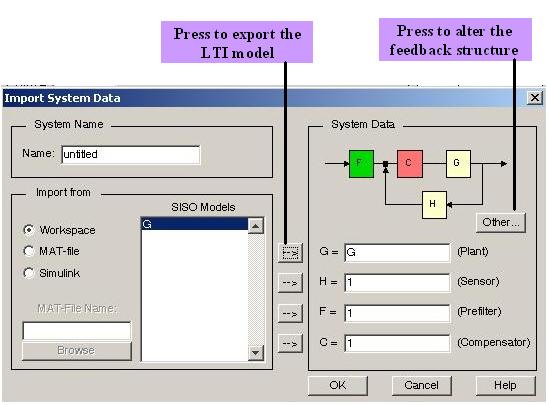
The following MATLAB commands create the transfer function num=4500; den=[1 361.2 0]; G=tf(num,den) 3. Create the closed-loop model for the SISO Design Tool: Choose Import� under the File menu in the SISO Design Tool window to display the window shown in Fig. M7.19. LTI objects can be selected from the SISO Models list and can be exported to one of the blocks of the system by pressing the right-facing arrow next to the selected block ( G, H, F, or C ) located in the section of the window labeled System Data. Press the Other� button to rotate through a selection of feedback structures and select the desired configuration. Alternatively, this can also be done by pressing the FS button on the bottom right corner of closed-loop block diagram in the SISO Design Tool window (Fig. M7.18). Root locus and Bode diagrams will change immediately to reflect the changes in the feedback structure (Fig. M7.20). LTI transfer function generating command, tf(num,den), can also be supplied directly into the spaces for transfer functions in Fig. M7.19.
Fig. M7.18 SISO Design Tool window
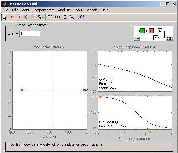
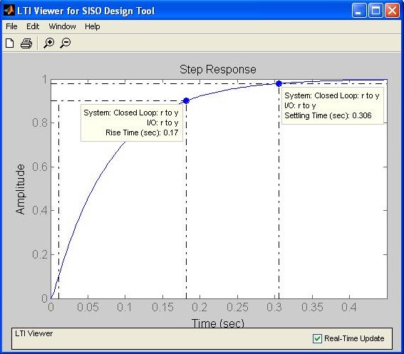
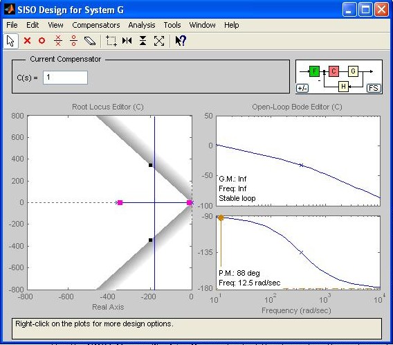
4. Interact with the SISO Design Tool: After the Import System Data window closes, the SISO Design Tool window now contains the root locus and Bode plots for the system as shown in Fig. M7.20. In this example, we have considered the open-loop system given by Under the Analysis menu, select the desired response to open the LTI Viewer for SISO Design Tool window (Fig. M7.21). Right-click on the LTI Viewer for SISO Design Tool and choose desired Plot Types, Systems, and Characteristics.
Fig. M7.19 Import System Data Window
With gain changes, you can read the gain and phase margins and gain crossover and phase crossover frequencies at the bottom of the Bode magnitude and phase plots. Also, at the bottom of the Bode magnitude plot, you are told whether or not the closed-loop system is stable.
Fig. M7.20 Root locus and Bode plots of G in SISO Design Tool window
Fig. M7.21 LTI Viewer for SISO Design Tool window
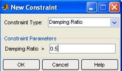
5. Design constraints: Design constraints may be added to your plots. These constraints may be selected by right-clicking a respective plot and selecting Design Constraints. To put new constraints, choose New� and to edit existing constraints, choose Edit� . For example, Fig.M7.22 shows the selection of design constraint: damping ratio=0.5. On pressing OK, indicators appear identifying portions of the root locus where the damping ratio is less than 0.5(shaded gray), equal to 0.5(damping line), and greater than 0.5( Fig.M7.23 ). Note the change made in axes limits in this figure with respect to Fig.M7.20 using the Property Editor (the description of the Property Editor is given in the next step).
Fig. M7.22 Adding design constraints
Fig.M7.23 Adding design constraints
6. Properties: Right-clicking in a plot's window and selecting Properties� displays the Property Editor window. From this window, some of the properties of the plot such as axes labels and limits can be controlled. Try exploring various options available with root locus and Bode plot properties editor. 7. Add poles, zeros, and compensators: Poles and zeros may be added from the
SISO Design Tool
window toolbar shown in Fig. M7.23. Let your mouse pointer rest on the button for a few seconds to see the functionality of the button in the form of screen tips.
Add real pole; Add real zero;
Add complex pole; Add complex zero; Delete pole/zero; .....
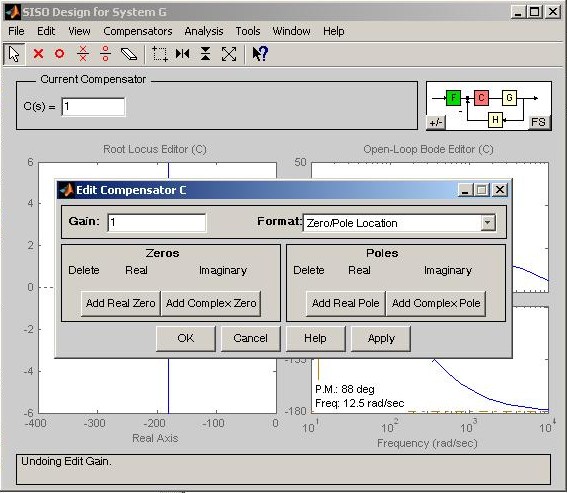
functions are available. 8. Editing compensators and prefilters: The pole and zero values of the compensators and prefilters can be edited in several ways. The most convenient is to click on C or F blocks in the block diagram representation in top-right corner of the SISO Design Tool window (Fig. M7.23).This operation will open prefilter or compensator editor window shown in Fig. M7.24. Desired real/complex zero/pole locations can be edited here. The same windows can also be opened by following Compensators In control systems design, we use compensators of the form that alter the roots of the characteristic equation of the closed-loop system. However, the closed-loop transfer function, M(s), will contain the zero of D(s) as a zero of M(s).This zero may significantly affect the response of the system M(s). We may use a prefilter F(s) to reduce the effect of this zero on M(s). For example, if we select we cancel the effect of the zero without changing the dc gain. Prefilters may be employed with lead/PD compensation.
Fig. M7.24 Editing compensators and prefilters
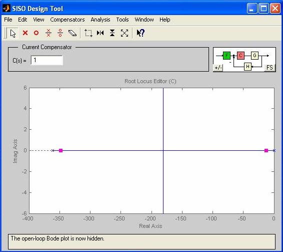
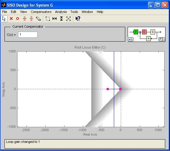
Example 7.4 Consider a plant with the following transfer function: We will design a cascade controller using SISO Design Tool in interactive mode, so that the unity feedback closed-loop system meets the following criteria (refer Kuo and Golnaraghi(2003)): Steady-state error due to unit-ramp input Maximum overshoot Rise time Settling time The first step is to import the model into SISO Design Tool. System transfer functions can be imported in SISO Design Tool by clicking on File and then going to Import� Before executing this sequence, create transfer function G in MATLAB Command Window: num=4500; den=[1 361.2 0]; G=tf(num,den) In order to examine the system performance, we start by using a proportional controller. The system root locus can be obtained by clicking on View in the main menu and then selecting Root Locus only. Fig. M7.25 shows the root locus of the system. The plot is for K =1(by default).
Fig. M7.25
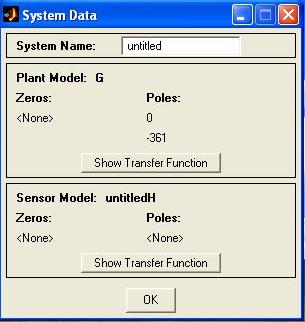
In order to see the poles and zeros of G and H , go to the View menu and select System Data, or alternatively, double click the block G or H in the top-right corner of the block diagram in the SISO Design Tool window. The System Data window is shown in Fig.M7.26.
Fig. M7.26
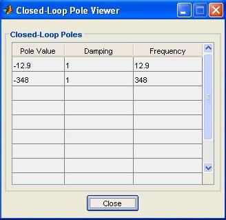
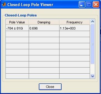
You may obtain the closed-loop system poles by selecting Closed-Loop Poles from the View menu. Closed-loop poles are given in Fig.M7.27.
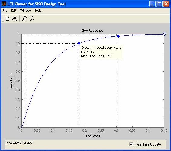
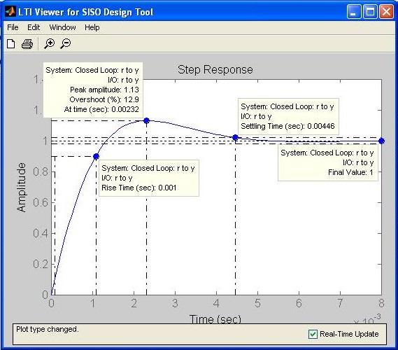
Fig. M7.27 In order to see the closed-loop system time response to a unit-step input, select the Response to Step Command in the Analysis main menu. With specific selections made in Systems and Characteristics submenus, we generate Fig. M7.28, which shows the unit step response of the closed-loop system with unity gain controller, i.e. , K= 1.
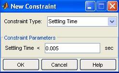
Fig. M7.28 As a first step to design a controller, we use the built-in design criteria option within the SISO Design Tool to establish the desired closed-loop poles regions on the root locus. To add the design constraints, use the Edit menu and choose the Root Locus option. Select New to enter the design constraints. The Design Constraints option allows the user to investigate the effect of the following: We will use the settling time and the percent overshoot as primary constraints. After designing a controller based on these constraints, we will determine whether the system complies with the rise time constraint or not. Figure M7.29 shows the addition of settling time constraint. Peak overshoot constraint is added on similar lines.
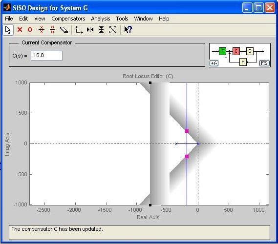
Fig. M7.29 Figure M7.30 shows the desired closed-loop system pole locations on the root locus after inclusion of the design constraints (Note that the scale has been modified by following Right click --> Properties --> Limits. Left-clicking anywhere inside plot will remove the black squares on the zeta lines). Obviously, closed-loop poles of the system for K = 1 are not in the desired area. Note the definition of the desired area: the vertical gray bar signifies the boundary for that portion of the root locus where the settling time requirement is not met; and the gray bars on damping lines signify the boundary for that portion of the root locus where the peak overshoot requirement is not met. Changing K will affect the pole locations. In the Root Locus window, C(s) represents the controller transfer function. Fig.M7.30 corresponds to C(s) = K = 1 . Hence, if C(s) is increased, the effective value of K increases, forcing the closed-loop poles to move together on the real axis, and then ultimately to move apart to become complex. See Fig. M7.31 wherein K= 16.8 gives closed-loop poles on the damping lines. However, the settling time requirement is not met.
Fig. M7.30
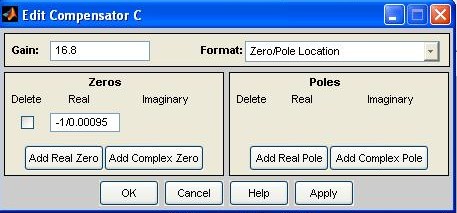
Fig. M7.31 The closed-loop poles of the system must lie to the left of the boundary imposed by the settling time(Fig.M7.31). Obviously, it is impossible to use the proportional controller (for any value of K ) to move the poles of the closed-loop system farther to the left-hand plane. However, a PD controller C(s)= K (1+ sTD ) may be used to accomplish this task. The zero s = - 1/ TD of the compensator has to be placed far into the left half plane to move the root-locus plot to the left. We have tried various values: s = - 1/0.0005; - 1/0.001; - 1/0.0015; - 1/0.002,... The value s = -1/0.00095 gives satisfactory results. To add a zero to the controller, click the C block in the block diagram in top-right corner of Fig. M7.31. Fig.M7.32 shows the Edit Compensator window and how the PD controller is added:
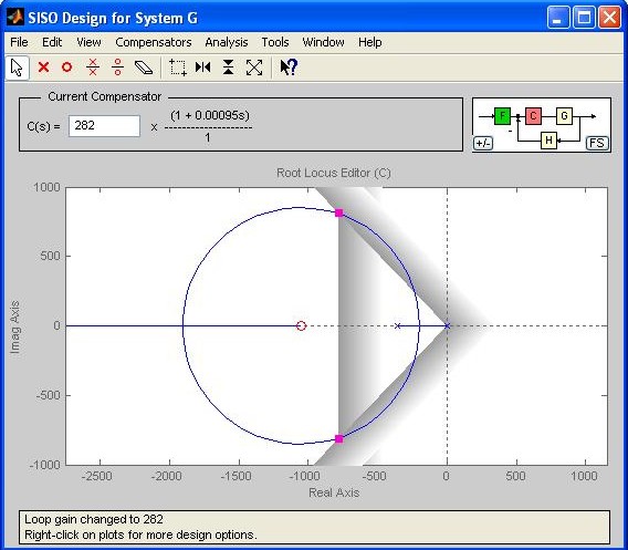
Fig. M7.32 Figure M7.33 shows the plot for s= - 1/0.00095. Note that the closed-loop poles have been dragged to the desired locations. The value of K that achieves the desired dominent closed-loop poles is 282. This value of K forces the closed-loop poles to the desired region. The system closed-loop poles are shown in Fig. M7.34.
Fig. M7.33
Fig. M7.34 The step response of the controlled system in Fig. M7.35 shows that the system has now complied with all design criteria.
Fig. M7.35
|
|