Stability Analysis on Root Locus Plots
Root Locus Analysis
In the following, we provide brief description of powerful MATLAB commands for root locus analysis. The reader may wonder why the instructors emphasize learning of hand calculations when powerful MATLAB commands are available. For a given set of open-loop poles and zeros, MATLAB immediately plots the root loci. Any changes made in the poles and zeros, immediately result in new root loci and so on.
Depending on our background and aptitude, we may, after a while, begin to make some sense of the patterns. May be we finally begin to formulate a set of rules that enables us to quickly make a mental sketch of the root locus the moment the poles and zeros appear. In other words, by trial-and-error, we find the rules of the root locus.
Through the systematic formulation of set of rules of the root locus, we look for the clearest, and simplest explanation of the dynamic phenomena of the system. The rules of the root locus give us a clear and precise understanding of the endless patterns that can be created by an infinite set of characteristic equations. We could eventually learn to design without these rules, but our level of skill would never be as high or our understanding as great. This is true of other analysis techniques also such as Bode plots, Nyquist plots, Nichols charts, and so on, covered later in the course.
MATLAB allows root locus for the characteristic equation
1 + G (s)H(s) = 0
to be plotted with the rlocus(GH) command. Points on the root loci can be selected interactively (placing the cross-hair at the appropriate place) using the [K,p] = rlocfind(GH) command. MATLAB then yields the gain K at that point as well as all the poles p that have that gain. The root locus can be drawn over a grid generated using the sgrid (zeta, wn) command, that allows constant damping ratio zeta and constant natural frequency wn curves. The command rlocus (GH, K) allows us to specify the range of gain K for plotting the root locus. Also study the commands [p,K]=rlocus(GH) and [p]=rlocus(GH,K) using MATLAB online help.
Example M6.1
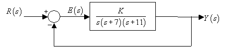
Consider the system shown in the block diagram of Fig. M6.1.
Fig. M6.1
The characteristic equation of the system is
1 + G(s) = 0
with
![]()
The following MATLAB script plots the root loci for
s = tf('s');
G = 1/(s*(s+7)*(s+11));
rlocus(G);
axis equal;
Clicking at the point of intersection of the root locus with the imaginary axis gives the data shown in Fig. M6.2. We find that the closed-loop system is stable for K < 1360; and unstable for K > 1360.
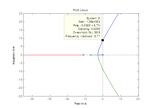
Fig. M6.2
Fig. M6.3 shows step responses for two values of K .
>> K = 860;
>> step(feedback(K*G,1),5)
>> hold;
% Current plot held
>> K = 1460;
>> step(feedback(K*G,1),5)
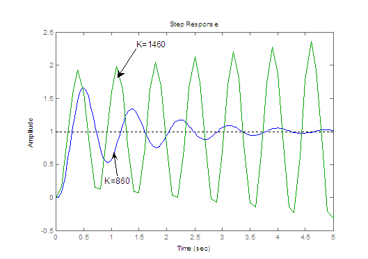
Fig. M6.3
Example M6.2
Consider the system shown in Fig. M6.4.
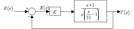
Fig M6.4
The plant transfer function G(s) is given as as
![]()
The following MATLAB script plots the root locus for the closed-loop system.
clear all;
close all;
s = tf('s');
G = (s+1)/(s*(0.1*s-1));
rlocus(G);
axis equal;
sgrid;
title('Root locus for (s+1)/s(0.1s-1)');
[K,p]=rlocfind(G)
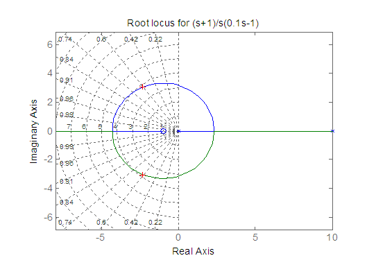
Fig M6.5
selected_point =
-2.2204 + 3.0099i
K =
1.4494
p =
-2.2468 + 3.0734i
-2.2468 - 3.0734i
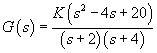
Example M6.3
For a unity feedback system with open-loop transfer function
a root locus plot shown in Fig. M6.6 has been generated using the following MATLAB code.
s = tf('s');
G = (s^2-4*s+20)/((s+2)*(s+4));
rlocus(G);
zeta = 0.45;
wn = 0;
sgrid(zeta,wn);
Properly redefine the axes of the root locus using Right click --> Properties --> Limits.
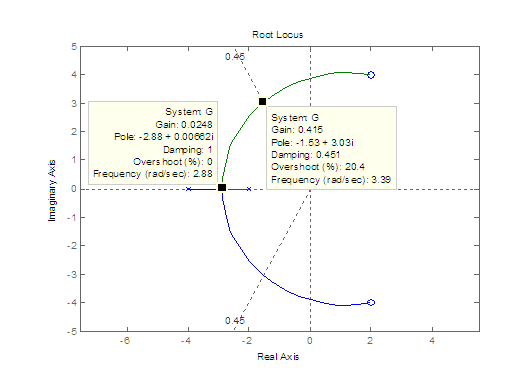
Fig. M6.6
Clicking on the intersection of the root locus with zeta=0.45 line gives the system gain K = 0.415 that corresponds to closed-loop poles with
Clicking on the intersection of the root locus with the real axis gives the breakaway point and the gain at that point.