MATLAB MODULE 5

Time Response Characteristics and LTI Viewer

Time Response Characteristics in SIMULINK window

Example M5.3

Consider a unity feedback, PID controlled system with following parameters:

Plant transfer function:

PID controller transfer function:

Reference input:

A Simulink block diagram is shown in Fig. M5.13.

 

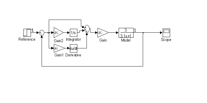
Fig. M5.13 (download)

The Simulink model inputs a step of 30 to the system.

Time response characteristics of the model developed in Simulink can be obtained by invoking the LTI Viewer directly from the Simulink. LTI Viewer for Simulink can be invoked by following Tools -- Control Design -- Linear Analysis as shown in Fig. M5.14.

 

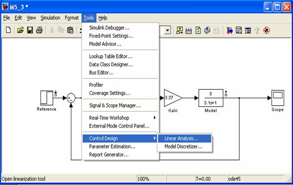
Fig. M5.14

This opens Control and Estimation Tools Manager shown in Fig. M5.15.

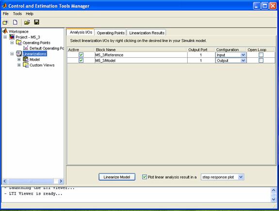
Fig. M5.15

Select linearization input-output points by right clicking on the desired line and selecting Linearization Points in your Simulink model. Fig. M5.16 explains the selection of input point. Similarly output point has been selected. Once input-output linearization points appear in the Control and Estimation Tools Manager window, click on the Linearize Model at the bottom of the window (Fig. M.5.15). The type of response can be selected from the drop down menu just near the Linearize Model button. Other linear analysis plots available are: Bode, Impulse, Nyquist, Nichols, Bode magnitude plot, and pole-zero map.

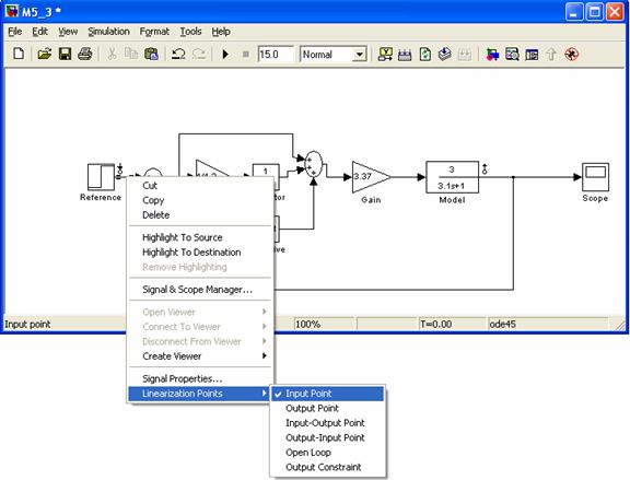
Fig. M5.16

The step response with the characteristics is shown in Fig. M5.17.

 

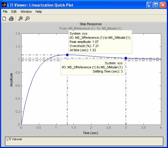
Fig. M5.17

Example M5.4

Consider a unity feedback, PI controlled system with following parameters:

Plant transfer function: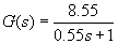

Plant deat-time: = 0.15 minutes

PI controller transfer function: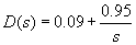

Actuator saturation characteristic: Unit slope; maximum control signal =1.7.

Reference input:

A Simulink block diagram is shown in Fig. M5.18. PID controller block is available in Additional Linear block set in Simulink Extras block library. The parameters of PID controller block have been set as : P = 0.09, I = 0.95, and D = 0.

 

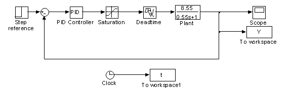
Fig. M5.18 (download)  

 

We can invoke LTI Viewer to determine the time response characteristics of the system of Fig. M5.18. However, LTI Viewer will linearize the system and then plot the characteristics. An alternative is to transfer the output response data to workspace using To Workspace block and then generate the time response using the plot command. A MATLAB code can then be written to determine the required characteristics. The following code gives settling time, peak overshoot, and peak time for the output response data of Fig. M5.18.

time = t.signals.values;

y = Y.signals.values;

plot(time,y);

title('Step response');

xlabel('Time (min)');

ylabel('Output');

ymax = max(y);

step_size = 10;

peak_overshoot = ((ymax-step_size)/step_size)*100

index_peak = find(y == ymax);

peak_time = time(index_peak)

s = length(time);

while((y(s)>=0.95*step_size) & (y(s)<=1.05*step_size))

s = s-1;

end

settling_time = time(s) 

The MATLAB responds with Fig. M5.19 and the following characteristics.

peak_overshoot =

39.0058

peak_time =

1.9339

settling_time =

5.9739

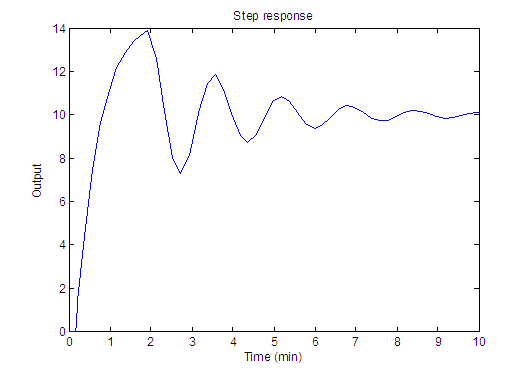
Fig. M5.19