MATLAB MODULE 2

Control System Toolbox and Symbolic Math Toolbox

Control System Toolbox

Control System Toolbox is a collection of commands to be used for control systems' analysis and design. We will be using only some of these commands, because of the limited nature of course profile. Description of these commands will be distributed in different modules.

In this module, we will present commands related to transfer functions and system responses. To see all the commands in the Control System Toolbox and their functionalities, type help control in the MATLAB command window. MATLAB will respond with

>> help control

Control System Toolbox
Version 6.0 (R14) 05-May-2004

General.
ctrlpref - Set Control System Toolbox preferences.
ltimodels - Detailed help on the various types of LTI models.
ltiprops - Detailed help on available LTI model properties.

Creating linear models.
tf - Create transfer function models.
zpk - Create zero/pole/gain models.
ss, dss - Create state-space models.
frd - Create a frequency response data models.
filt - Specify a digital filter.
lti/set - Set/modify properties of LTI models.

Data extraction.
tfdata - Extract numerator(s) and denominator(s).
zpkdata - Extract zero/pole/gain data.
ssdata - Extract state-space matrices.
dssdata - Descriptor version of SSDATA.
frdata - Extract frequency response data.
lti/get - Access values of LTI model properties.

Conversions.
tf - Conversion to transfer function.
zpk - Conversion to zero/pole/gain.
ss - Conversion to state space.
frd - Conversion to frequency data.
chgunits - Change units of FRD model frequency points.
c2d - Continuous to discrete conversion.
d2c - Discrete to continuous conversion.
d2d - Resample discrete-time model.

System interconnections.
append - Group LTI systems by appending inputs and outputs.
parallel - Generalized parallel connection (see also overloaded +).
series - Generalized series connection (see also overloaded *).
feedback - Feedback connection of two systems.
lft - Generalized feedback interconnection (Redheffer star product).
connect - Derive state-space model from block diagram description.

System gain and dynamics.
dcgain - D.C. (low frequency) gain.
bandwidth - System bandwidth.
lti/norm - Norms of LTI systems.
pole, eig - System poles.
zero - System (transmission) zeros.
pzmap - Pole-zero map.
iopzmap - Input/output pole-zero map.
damp - Natural frequency and damping of system poles.
esort - Sort continuous poles by real part.
dsort - Sort discrete poles by magnitude.
stabsep - Stable/unstable decomposition.
modsep - Region-based modal decomposition.

Time-domain analysis.
ltiview - Response analysis GUI (LTI Viewer).
step - Step response.
impulse - Impulse response.
initial - Response of state-space system with given initial state.
lsim - Response to arbitrary inputs.
gensig - Generate input signal for LSIM.
covar - Covariance of response to white noise.

Frequency-domain analysis.

ltiview - Response analysis GUI (LTI Viewer).
bode - Bode diagrams of the frequency response.
bodemag - Bode magnitude diagram only.
sigma - Singular value frequency plot.
nyquist - Nyquist plot.
nichols - Nichols plot.
margin - Gain and phase margins.
allmargin - All crossover frequencies and related gain/phase margins.
freqresp - Frequency response over a frequency grid.
evalfr - Evaluate frequency response at given frequency.
frd/interp - Interpolates frequency response data.

Classical design.
sisotool - SISO design GUI (root locus and loop shaping techniques).
rlocus - Evans root locus.

Pole placement.
place - MIMO pole placement.
acker - SISO pole placement.
estim - Form estimator given estimator gain.
reg - Form regulator given state-feedback and estimator gains.

LQR/LQG design.
lqr, dlqr - Linear-quadratic (LQ) state-feedback regulator.
lqry - LQ regulator with output weighting.
lqrd - Discrete LQ regulator for continuous plant.

kalman - Kalman estimator.
kalmd - Discrete Kalman estimator for continuous plant.
lqgreg - Form LQG regulator given LQ gain and Kalman estimator.
augstate - Augment output by appending states.

State-space models.
rss, drss - Random stable state-space models.
ss2ss - State coordinate transformation.
canon - State-space canonical forms.
ctrb - Controllability matrix.
obsv - Observability matrix.
gram - Controllability and observability gramians.
ssbal - Diagonal balancing of state-space realizations.
balreal - Gramian-based input/output balancing.
modred - Model state reduction.
minreal - Minimal realization and pole/zero cancellation.
sminreal - Structurally minimal realization.

Time delays.
hasdelay - True for models with time delays.
totaldelay - Total delay between each input/output pair.
delay2z - Replace delays by poles at z=0 or FRD phase shift.
pade - Pade approximation of time delays.

Model dimensions and characteristics.
class - Model type ('tf', 'zpk', 'ss', or 'frd').
size - Model sizes and order.
lti/ndims - Number of dimensions.
lti/isempty - True for empty models.
isct - True for continuous-time models.
isdt - True for discrete-time models.
isproper - True for proper models.
issiso - True for single-input/single-output models.
reshape - Reshape array of linear models.

Overloaded arithmetic operations.
+ and - - Add and subtract systems (parallel connection).
* - Multiply systems (series connection).
\ - Left divide -- sys1\sys2 means inv(sys1)*sys2.
/ - Right divide -- sys1/sys2 means sys1*inv(sys2).
^ - Powers of a given system.
' - Pertransposition.
.' - Transposition of input/output map.
[..] - Concatenate models along inputs or outputs.
stack - Stack models/arrays along some array dimension.
lti/inv - Inverse of an LTI system.
conj - Complex conjugation of model coefficients.

Matrix equation solvers.
lyap, dlyap - Solve Lyapunov equations.
lyapchol, dlyapchol - Square-root Lyapunov solvers.
care, dare - Solve algebraic Riccati equations.
gcare, gdare - Generalized Riccati solvers.
bdschur - Block diagonalization of a square matrix.

Demonstrations.
Type "demo" or "help ctrldemos" for a list of available demos.
control is both a directory and a function.
--- help for modeldev/control.m ---

MODELDEV/CONTROL

In this module, we will learn how to represent transfer functions in the MATLAB, partial fraction expansion of rational expressions, representation of transfer functions as LTI objects, and to obtain time domain responses of LTI systems. Important commands for this module are:

roots – Find polynomial roots
poly – Convert roots to polynomial
polyval – Evaluate polynomial value
conv – Convolution and polynomial multiplication
deconv – Deconvolution and polynomial division
residue – Partial-fraction expansion (residues)
tf – Creation of transfer functions or conversion to transfer functions
pole – Compute the poles of LTI models
zero – Transmission zeros of LTI systems
tfdada – Quick access to transfer function data
zpkdata – Quick access to zero-pole-gain data
pzmap – Pole-zero map of LTI models
zpk – Create zero-pole-gain models or convert to zero-pole-gain format
step – Step response of LTI models
impulse – Impulse response of LTI models
lsim – Simulate time response of LTI models to arbitrary inputs
gensig – Periodic signal generator for time response simulations with lsim

Polynomials

Consider a polynomial ‘s ³ +3 s ² +4', to which we attach the variable name p. MATLAB can interpret a vector of length n +1 as the coefficients of an n ^th -order polynomial. Coefficients of the polynomial are interpreted in descending powers. Thus, if the polynomial is missing any coefficient, we must enter zeros in the appropriate places in the vector. For example, polynomial p can be represented by the vector [1 3 0 4] in MATLAB. For example:

>> p=[1 3 0 4]

p =

1 3 0 4

Roots of the polynomial can be obtained by roots command.

>> r=roots(p)

r =

  -3.3553          

   0.1777 + 1.0773i

   0.1777 - 1.0773i

Given roots of a polynomial in a vector, a vector of polynomial coefficients can be obtained by the command poly.

>> p=poly(r)

p =

    1.0000     3.0000     0.0000     4.0000   

Use the command polyval(p, s) to evaluate the polynomial represented by vector p at arbitrary value of s. For example, to evaluate the polynomial 's ³ +3 s ² +4' at , type

>> polyval(p,sqrt(2))

ans =

   12.8284

The product of two polynomials is found by taking the convolution of their coefficients. The function conv will do this for us. Consider an example of multiplying polynomial ‘s 3 +3 s 2 +4' with ‘s +2':

>> p1=[1 3 4];

>> p2=[1 2];

>> p3=conv(p1,p2)

p3 =

     1      5     10      8

The function deconv divides two polynomials and returns quotient as well as the remainder polynomial.

>> [q,r]=deconv(p1,p2)

q =

     1      1

r =

     0      0      2

where q is the quotient and r is the remainder polynomial.

Transfer Functions

Transfer functions can be represented in MATLAB as LTI (Linear Time Invariant) objects using numerator and denominator polynomials. Consider the transfer function given by   It can be represented in MATLAB as:

>> num = [1 1];

>> den = [1 3 1];

>> G = tf(num,den)

 

Transfer function:

    ..s + 1
-----------------
s^2 + 3 s + 1

 

Example M2.2

The function conv has been used to multiply polynomials in the following MATLAB session for the transfer function

 

 

>> n1 = [5 1];

>> n2 = [15 1];

>> d1 = [1 0];

>> d2 = [3 1];

>> d3 = [10 1];

>> num = 100*conv(n1,n2);

>> den = conv(d1,conv(d2,d3));

>> GH = tf(num,den)

 

Transfer function:

7500 s^2 + 2000 s + 100
-----------------------------------
....30 s^3 + 13 s^2 + s

 

 

To learn more about LTI objects given by tf, type ltimodels tf in MATLAB command window. Type ltiprops tf on MATLAB prompt to learn the properties associated with an LTI object represented by tf.

Transfer functions can also be entered directly in polynomial form as we enter them in the notebook using LTI objects. For example, observe the following MATLAB session.

>> s=tf('s') %Define 's' as an LTI object in polynomial form

Transfer function:

s

>> G1=150*(s^2+2*s+7)/[s*(s^2+5*s+4)] % Form G1(s) as an LTI transfer function

% in polynomial form.

Transfer function:

150 s^2 + 300 s + 1050
---------------------------------
......s^3 + 5 s^2 + 4s

 

>> G2=20*(s+2)*(s+4)/[(s+7)*(s+8)*(s+9)] % Form G2(s) as an LTI transfer

% function in polynomial form.

Transfer function:

.....20 s^2 +120 s + 160
------------------------------------
s^3 + 24 s^2 + 191s + 504

The commands pole and zero calculate the poles and zeros of LTI models.

>> pole(G1)

ans =

0

-4

-1

>> zero(G1)

ans =

-1.0000 + 2.4495i

-1.0000 - 2.4495i

To extract numerator and denominator polynomials, use the function tfdata .

>> [num,den]=tfdata(G,'v')

num =

0 1 1

den =

1 3 1

To extract zeros and poles of transfer function simultaneously, use the function zpkdata .

>> [z,p]=zpkdata(G,'v')

z =

-1

p =

-2.6180

-0.3820

If we know zeros and poles of the system with gain constant, the transfer function of LTI system can be constructed by zpk command. For example, to create a unity gain transfer function G3(s) with zero at -1 and two poles at -2.618 and -0.382, follow the MATLAB session given below.

>> G3=zpk(-1,[-2.618 -0.382],1)

Zero/pole/gain:

          (s+1)
---------------------------
(s+2.618)(s+0.382)

The polynomial transfer function created with tf can be converted to zero-pole-gain model by the command zpk and vice versa . The following MATLAB session gives the zero-pole-gain format of LTI system represented by G(s).

>> zpk(G)

Zero/pole/gain:

          (s+1)
---------------------------
(s+2.618)(s+0.382)

To observe the polynomial form of the transfer function G3(s), enter

>> tf(G3)

Transfer function:

          s+1
----------------------
    s^2 + 3s +1

To learn more about LTI objects given by zpk, type ltimodels zpk in MATLAB command window. Type ltiprops zpk on MATLAB prompt to learn the properties associated with an LTI object represented by zpk.

The function pzmap(G) plots the poles and zeros of the transfer function G(s) on complex plane. When used with two left hand side arguments, [p,z] = pzmap(G), the function returns the poles and zeros of the system in two column vectors p and z. For example:

System Response

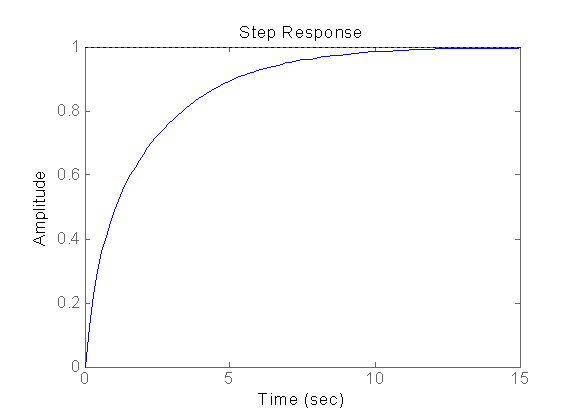
Step and impulse responses of LTI objects can be obtained by the commands step and impulse . For example, to obtain the step response of the system represented in LTI object G, enter

>> step(G)

The MATLAB response to this command is shown in Fig. M2.1.

 

Fig. M2.1

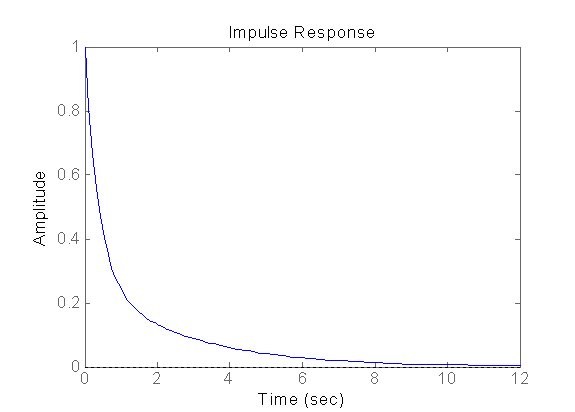
To obtain the impulse response, enter

>> impulse(G)

The MATLAB response to this command is shown in Fig. M2.2.

 

Fig. M2.2

Step and impulse response data can be collected into MATLAB variables by using two left hand arguments. For example, the following commands will collect step and impulse response amplitudes in yt and time samples in t.

[yt, t] = step(G)

[yt, t] = impulse(G)

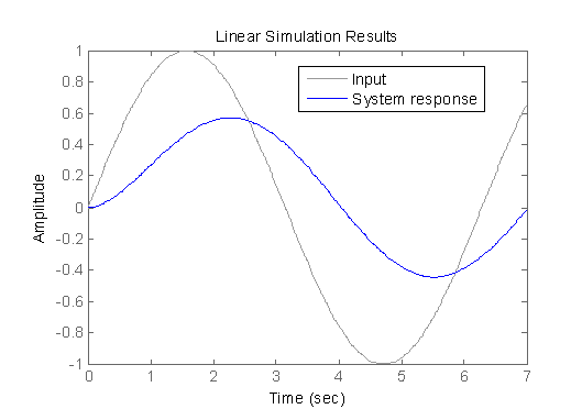
Response of LTI systems to arbitrary inputs can be obtained by the command lsim. The command lsim(G,u,t) plots the time response of the LTI model G to the input signal described by u and t. The time vector t consists of regularly spaced time samples and u is a matrix with as many columns as inputs and whose i^th -row specifies the input value at time t(i). Observe the following MATLAB session to obtain the time response of LTI system G to sinusoidal input of unity magnitude.

>> t=0:0.01:7;

>> u=sin(t);

>> lsim(G,u,t)

The response is shown in Fig. M2.3.

 

Fig. M2.3

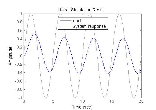
The function gensig generates periodic signals for time response simulation with lsim function. It can generate sine, square, and periodic pulses. All generated signals have unit amplitude. Observe the following MATLAB session to simulate G ( s ) for 20 seconds with a sine wave of period 5 seconds.

>> [u,t]=gensig( 'sin' ,5,20); %Sine wave with period 5 sec and duration 20 sec

>> lsim(G,u,t) %Simulate G(s) with u and t.

The response is shown in Fig. M2.4.

 

Fig. M2.4

Example M2.3

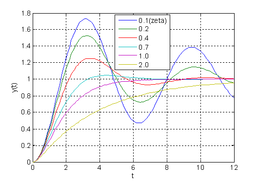
The following MATLAB script calculates the step response of second-order system

 

  with   and various values of

t=[0:0.1:12]; num=[1];  

zeta1=0.1; den1=[1 2*zeta1   1];

zeta2=0.2; den2=[1 2*zeta2   1];

zeta3=0.4; den3=[1 2*zeta3   1];

zeta4=0.7; den4=[1 2*zeta4   1];

zeta5=1.0; den5=[1 2*zeta5   1];

zeta6=2.0; den6=[1 2*zeta6   1];

[y1,x]=step(num,den1,t); [y2,x]=step(num,den2,t);

[y3,x]=step(num,den3,t); [y4,x]=step(num,den4,t);

[y5,x]=step(num,den5,t); [y6,x]=step(num,den6,t);

plot(t,y1,t,y2,t,y3,t,y4,t,y5,t,y6)

xlabel( 't' ), ylabel( 'y(t)' )

grid

Response through the above MATLAB script is shown in Fig M2.5.

Fig. M2.5 

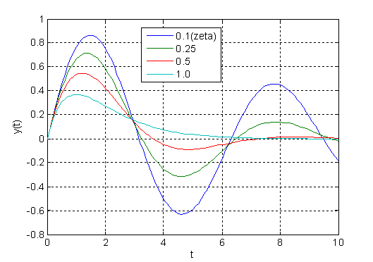
The following MATLAB script calculates the impulse response of second-order system

 

  with   and various values of

t=[0:0.1:10]; num=[1];  

zeta1=0.1; den1=[1 2*zeta1   1];

zeta2=0.25; den2=[1 2*zeta2   1];

zeta3=0.5; den3=[1 2*zeta3   1];

zeta4=1.0; den4=[1 2*zeta4   1];

[y1,x,t]=impulse(num,den1,t);

[y2,x,t]=impulse(num,den2,t);

[y3,x,t]=impulse(num,den3,t);

[y4,x,t]=impulse(num,den4,t);

plot(t,y1,t,y2,t,y3,t,y4)

xlabel( 't' ), ylabel( 'y(t)' )

grid

Response through the above MATLAB script is shown in Fig M2.6.

 

 

Fig. M2.6 

Right-clicking away from the curves obtained by step, impulse, and lsim commands brings up a menu. From this menu, various time-response characteristics can be obtained and plotted on the graph ( Discussion on time-response characteristics will appear later in Module 5).