Incremental-assignment model, in addition to the postulate that each trip-maker chooses a path so as to minimize his/her travel time, also assume that the travel time on a link varies with the flow on that link. Under such an assumption, the ideal way to assign traffic volume would be to assign a single trip to the road network assuming that the travel time on links during the assignment is constant. We could then update the travel times and repeat the process till all the trips are assigned. However, this procedure is not practical as any network would typically have a very large number of trips. The Incremental-assignment models, therefore, try to approximate this ideal process by dividing the total number of trips into a few smaller parts and then assigning each part with a constant link travel time.
The exact nature of the assignment model is presented through the following algorithm.
-
Step 0:
- Divide the entire trip-distribution matrix (or origin-destination matrix) into n
 smaller part matrices. Note that, the sum of all the part matrices should be equal to the actual trip-distribution matrix. smaller part matrices. Note that, the sum of all the part matrices should be equal to the actual trip-distribution matrix.
Set counter  . .
Set  for all a. for all a.
(Also note that in the following,  refers to the number of trips from i to j as per the refers to the number of trips from i to j as per the  part matrix.) part matrix.)
- Step 1:
- Set
 for all links. for all links.
Assuming
 as the link travel times, assign the trips of the part matrix using all-or-nothing assignment technique. Store the link volumes obtained from the all-or-nothing assignment technique as as the link travel times, assign the trips of the part matrix using all-or-nothing assignment technique. Store the link volumes obtained from the all-or-nothing assignment technique as  . .
- Step 2:
- Update the link volumes using
  . .
- Step 3:
- If
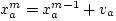
 then report as as xa and Stop. Else, set m = m + 1and go to Step 1. then report as as xa and Stop. Else, set m = m + 1and go to Step 1.
Example
For the network shown in Figure 6 and the trip distribution matrix given in Table 5 determine the link flows using the incremental assignment technique. The link travel times,  , are given by: , are given by: 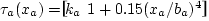 The link number, the The link number, the  value, and the value, and the  value, for a particular link are mentioned as value, for a particular link are mentioned as
 on the links. Divide the trip-distribution matrix into four parts in the ratio 40:30:20:10. on the links. Divide the trip-distribution matrix into four parts in the ratio 40:30:20:10.
Figure 6: Network for example problem on incremental assignment technique.
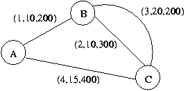 |
Table 5: Trip distribution matrix for the example problem in incremental assignment model.
Origin zone |
Destination zone |
A |
B |
C |
A |
0 |
250 |
150 |
B |
250 |
0 |
400 |
C |
150 |
400 |
0 |
Solution
Step 0
The trip distribution matrix is divided into the following four (i.e., n =4) parts:
Part 1 matrix |
Part 2 matrix |
Origin
zone |
Destination zone |
|
Origin zone |
Destination zone |
A |
B |
C |
|
A |
B |
C |
A |
0 |
100 |
60 |
|
A |
0 |
75 |
45 |
B |
100 |
0 |
160 |
|
B |
75 |
0 |
120 |
C |
60 |
160 |
0 |
|
C |
45 |
120 |
0 |
Part 3 matrix |
|
Part 4 matrix |
Origin
zone |
Destination zone |
|
Origin
zone |
Destination zone |
A |
B |
C |
|
A |
B |
C |
A |
0 |
50 |
30 |
|
A |
0 |
25 |
15 |
B |
50 |
0 |
80 |
|
B |
25 |
0 |
40 |
C |
30 |
80 |
0 |
|
C |
15 |
40 |
0 |
Set counter m =1.
Set  , ,  , ,  , and , and  . .
Step 1
Set ,  , ,  , and , and  and and 
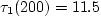
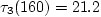
Using Part 1 matrix,  mins, mins,  mins, and mins, and  mins, and mins, and  , and all-or-nothing assignment the following values for , and all-or-nothing assignment the following values for  are obtained: are obtained:
 , ,  , , and , , and  . .
Step 2
Using  and the following quantities are obtained: and the following quantities are obtained:
 , ,  , and , and  , and , and  . .
Step 3
Since
 , set m = 2 and go to Step 1. , set m = 2 and go to Step 1.
Step 1
Set ,  , and . , and .
Using Part 2 matrix,
 mins., mins., 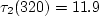 mins., mins., mins, and mins, and
 mins., and all-or-nothing assignment, the following values for are obtained: mins., and all-or-nothing assignment, the following values for are obtained:
 , ,  , and , and  . .
Step 2:
Using  and the following quantities are obtained: and the following quantities are obtained:
 , ,  , and , and  and and  . .
Step 3 :
Since
, set  , set m = 3 and go to Step 1. , set m = 3 and go to Step 1.
Step 1:
Set , , , and .
Using Part 3 matrix,
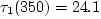 mins, mins, 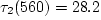 mins, mins,  mins, and mins, and 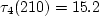 mins, and all-or-nothing assignment the following values for are obtained:
 , , , ,  and and  . .
Step 2 :
Using  and , the following quantities are obtained: and , the following quantities are obtained:
 , ,  , ,  and and  . .
Step 3:
Since
set  set m = 4 and go to Step 1. set m = 4 and go to Step 1.
Step 1 :
Set , , and .
Using Part 4 matrix, 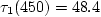 mins, mins,
 mins,and mins,and 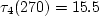 min,
and and all-or-nothing assignment the following values for are obtained: min,
and and all-or-nothing assignment the following values for are obtained:
, ,  and and  . .
Step 2:
Using  and , the following quantities are obtained: and , the following quantities are obtained:
 , ,  , ,  and and  . .
Step 3 :
Since
 , report , report
 , , 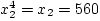 , ,
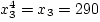 , and , and 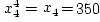 . .
Discussion: Although the incremental-assignment technique overcomes the shortcoming of the all-or-nothing assignment technique by incrementally assigning the entire trip-distribution matrix and updating the link travel times with flow, it still suffers from a major drawback. Despite the fact that traffic assignment is an outcome of the route choice behaviour of humans, the incremental-assignment technique does not have any behavioral basis and therefore remains more of a computational technique than a mechanism of traffic assignment which mirrors the route choice behaviour of humans.
|