| Friction factor |
| |
The friction factor is a dimensionless number, which provides an idea about the magnitude of shear stress produced by a solid boundary as fluid flows. This is defined as the ratio of shear stress at the wall and the kinetic energy head of the fluid,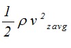 . Here, ρ is the density and  is the average velocity of fluid. The friction factor is thereby defined as |
| |
|
where,  is the shear force per unit area on the wall of the tube. This may be calculated as shown below |
| |
|
Here, first minus sign is used as the inside surface of the tube wall has outer normal in the negative r direction and second minus sign is used because  is treated here as momentum flux. If is
treated
as actual shear force then positive sign would have to be taken. For fully developed laminar flow, the velocity profile is parabolic and is given by |
| |
|
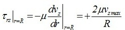
| Evaluating the velocity gradient at the wall (r=R), we have |
| |
|
| Thus, the shear stress
considered
as momentum flux is given by |
| |
|
| |
| or |
| |
|
| |
| The friction factor may now be calculated as shown below |
| |
|
| |
| or |
| |
|
| |
| Equation (11.7) shows that the friction factor in laminar flow region depends only on the Reynolds number. Clearly, the friction factor is also a dimensionless number. |
| |
| Friction factor in turbulent flow |
| |
|
Fig 11.1 Smooth and rough surface of pipe |
| |
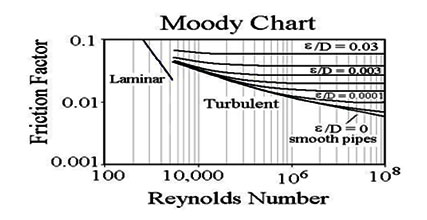
| In turbulent flow, the friction factor also depends on the surface of the pipe. A rough pipe leads to higher turbulence than a smoother pipe, so that the friction factor for smoother pipes is less than that for rougher pipes. The ratio of surface roughness height (∈) to pipe diameter (D) is used to quantify the “roughness” of the pipe surface. In practice, the shear stress on the wall may be calculated by measuring the pressure drop across the pipe for a given flow rate. Thus, friction factor may be calculated as the function of
Reynolds
number and plotted on a log-log plot for a given surface roughness. The curves are different for different surface roughness as shown in figure. (11.2). The collection of these f-Re plots is called Moody Chart as shown in figure below, and can be used for estimating the friction factor for given flow parameters. |
| |
|
|
Ref: http://www.brighthub.com/engineering/civil/articles |
| |
| Solution of some more fluid flow problems by shell momentum balance approach |
| |
| In this section, we solve a few more fluid mechanics problems in simple geometries using the shell momentum balance approach. The detail procedure, which was also used in previous example, is outlined below. |
| |
1) Make a diagram of the flow geometry with the appropriate coordinate system |
| |
2) Specify all
necessary
assumptions |
| |
| 3) Intuitively assume the velocity profile |
| |
| This is an important step for solving these problems. In laminar flow, the fluid flows in parallel layer without mixing. Thus, it is easy to guess the non-zero components of velocities by intuition. |
| |
| 4) Apply of the equation of
continuity
to modify the velocity profile |
| |
| 5) Determine the non-zero shear stress component(s) |
| |
| Since the shear stress components depend on the velocity profile, the non-zero shear stress components may now be determine. |
|
6) Determine control volume and make shell momentum balance for the control volume |
| |
Draw control volume in system diagram according to system shape, size and problem statement. The selection of proper control volume is very important to solve problem correctly. The control volume should be select in such way that it can be easily integrated for whole system. The differential length of control volume should be taken in direction of changing velocity.
Write momentum balance equation for the control volume. The shear stress may be considered as shear force or as momentum flux, both provide the same results as shown in previous example
. Write
down all surface and body force acting on the fluid carefully.
Finally
obtain a
appropriate differential
equation and
integrate.
|
| |
| 7) Boundary conditions |
| |
| Use
appropriate
boundary conditions which help us to determine the constant of integration in above step. |
| |
Falling film on an inclined flat surface
|
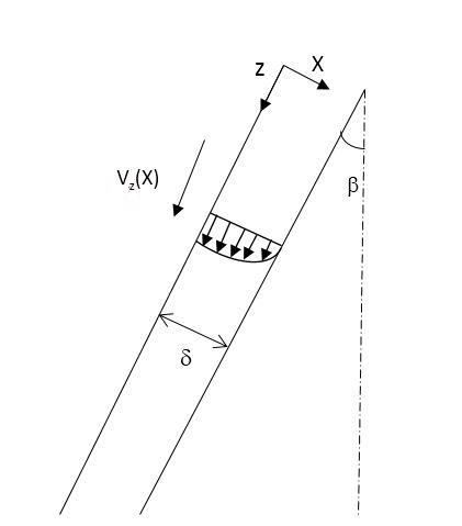
| An inclined surface of length L and width W is situated at an angle Β to the vertical direction as shown in Fig. (11.3). A Newtonian fluid is freely falling on the surface as a film of thickness δ. Assuming the flow to be laminar, determine the velocity profile, flow rate and shear force on the surface by the fluid. |
| |
| Solution |
|
Fig 11.3 Laminar flow on an inclined surface |
| |
| Assumptions |
| |
- Constant density, viscosity
- Steady state
- Laminar flow (simple shear flow)
- Fully developed flow
- Newton's law of viscosity is applicable
|
| |
| Assume velocity profile
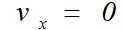
The fluid is flowing in the z direction, hence only the z component of velocity is non-zero. Thus, we may assume |
| |
|
| |
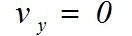
| We may further assume that vz does not depends upon y coordinate. Since the flow is steady, vz does not depend on time. Thus, |
| |
| |
|
| Using the equation of continuity in the cartesian coordinates for constant fluid density, we have |
| |
|
| |
| which reduces to |
| |
|
| |
| Equation (11.11) indicates that vz does not depend on the z coordinate. Thus, |
| |
|
| |
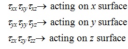
| There are nine components of the shear stress as shear force or momentum flux, namely |
| |
|
| |
Since vz is only the non-zero velocity, and also it is the function of x coordinate ,  is the only significant component of shear stress and we need to write momentum balance only in z direction. Because the pressure is same at both ends of the inclined plane, there is no pressure force on the fluid. Now, we can solve this problem by assuming shear stress as a shear force or shear stress as momentum flux. |
| |
Assuming  as momentum flux |
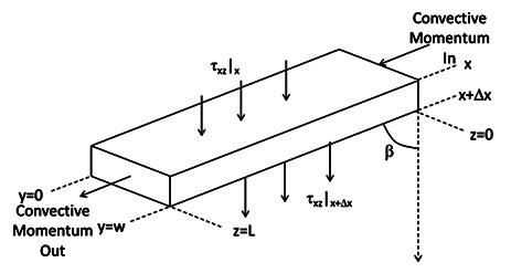
| Draw a control volume of length L, width W and differential thickness dx. |
| |
|
Fig 11.3 Control volume for falling film problem |
| |
| Momentum balance in x direction |
| |
| Rate of momentum flux entering CV due to viscous transport at |
| |
|
| |
| Rate of momentum flux leaving CV due to viscous transport at |
| |
|
| |
| Gravity force acting on fluid in z direction |
| |
|
| |
| Rate of momentum flux entering in CV due to convective transport |
| |
|
| |
| Rate of momentum flux leaving from CV due to convective transport |
| |
|
| |
| Now, when above terms are substituted for z-momentum balance, we obtain |
| |
|
| |
| Since the velocity vz does not depends on z coordinate, the first two terms
cancel
out and we obtain |
| |
|
| Dividing Equation (11.19) by volume of the control volume (LWΔx), we have |
| |
|
| |
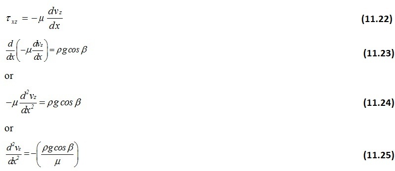
| As Δx→0 , The Equation (11.20)simplified to |
| |
|
| |
| The Newton’s law of viscosity (here, shear stress is defined as momentum flux) is given by |
| |
|
| |
| By integrating the Equation (11.25), we have |
| |
|
| or |
| |
|
| |
| The above equation requires two boundary conditions for determining c1 and c2. |
| |
| Boundary conditions |
| |
| 1 At x=0 the liquid surface is in contact with air where the shear stresses at both gas liquid phases should be equal. Thus, |
| |
|
| |
| Since both may be assumed Newtonian fluids, we have |
| |
|
| |
where ρg is the density and µg is the viscosity of air. Thus |
| |
|
| |
| Since, µg and ρg is much smaller than µ and ρ, and Equation (11.30) may be
approximately
written as |
| |
|
| |
| Substituting above boundary condition in Equation (11.26), we obtain |
| |
|
| |
| 2. At x=δ no slip boundary condition may be applied, i.e., |
| |
at  |
| |
| Thus, from Equation (11.27), we get |
| |
|
| |
| or |
| |
|
| |
| Finally the velocity profile is obtained as |
| |
|
| |
| or |
| |
|








 ,
 and